
!zip -r /content/drive/MyDrive/2024-01-09-Bauernproteste/2024-01-09-Images-Clean.zip mediaVisual Exploration
The previous chapter outlines some literature on images as data, emphasizing them importance of evaluation and contextualisation of computer vision applications due to biases inherent to our looking at images. This chapter introduces several tools and approaches for exploring visual material. These unsupervised approaches are useful for exploring image datasets. The first approaches, PixPlot and PicArrange are ready-made tools, they are easy to use and display results quickly. On the downside they offer limited options to manipulate the clustering of images (i.e. what features we are interested in). Therefore we take a look at commercial computer vision APIs as middle ground between setting up your own notebook for using object detection models, and the fully automated approaches above. We approach the labels using two clustering approaches in this chapter: Using network analysis and the modularity algorithm in Gephi finding communities, or using k-means to find k-clusters in our own notebook. The network analysis is based on Omena et al. (2021)’s manuals and publications. This approach is complex to reproduce for the sheer interest in image exploration (in contrast to Omena et al.’s interests in studying the web entity networks and their evolutions). The k-means approach offers an easier solution for clustering images based on labels provided by a vision API, while being compatible with Memespector, a GUI tool for multiple vision APIs. Finally we will explore BERTopic’s multimodal functionality: Using the vit-gpt2-image-captioning model, we generate captions for each image and use them for topic modeling. This captioning approach is one option, we will explore more options in union with image classification in the next session.
Note
I removed several code cells for rendering the results from the recipes below. The notebooks hosted on GitHub (links below the code and on the top-right) include these cells.
PixPlot
PixPlot is a visualization tool designed for clustering large numbers of images into a coherent projection. The tool uses Tensorflow’s Inception model to analyze image content and employs a custom WebGL viewer for visualization. This approach allows for the grouping of similar images, aiding in the identification of patterns and relationships within large image datasets.
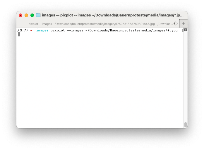
PixPlot requires a Python 3.7 environment, which can be set up using Anaconda. After setting up the environment, PixPlot can be installed via pip. For visualizing the results, a WebGL-enabled browser is necessary. The process involves running a simple command to process a directory of images, and then starting a web server to view the visualization. Take a look at the GitHub repository for instructions. The software is known for causing problems with newer MacBooks (based on the new M-Chips).

PixPlot has similarities with the k-means approach introduced in the next section. Both methods aim to categorize and cluster images based on their content. However, PixPlot automates this process by using an Inception model for image analysis and UMAP for dimensionality reduction, leading to the formation of clusters. For the approach below we first use the Google Vision API to retrieve a set of labels describing each images, and cluster afterwards. The manual approach is more difficult to start with, but possibly pays off as we progress towards image classification and the potential reuse of the labels retrieved from the API.
PicArrange

PicArrange helps to find images on your Mac computer much easier than ever before. Opposed to the Finder app, PicArrange can sort images not only by name or date, but also by content and color. This visual sorting mode allows to inspect and search large amounts of images much faster. You can also view visually sorted images from several directories at the same time, making it easy to find duplicate images.
Besides the visual sorting PicArrange offers a similarity search, thus allowing to find images similar to one or more example images. Image files can be deleted, copied or opened with Preview directly with PicArrange
Available at visual-computing.com, for macOS only.
Commercial Computer Vision APIs
Commercial services such as the Google Vision API and Microsoft Azure Vision provide an excellent starting point for exploring large visual datasets. This recipe is based on Omena’s work with labels and web entities from the Google Vision API (Omena et al. 2021). Utilizing tools like Memespector (Chao 2023), Table2Net, and Gephi, we can analyze image graphs without any programming knowledge. Subsequently, we apply the same labels in a matrix-based approach, clustering images using the k-means algorithm.
ImportantWarning: Black Boxes
When using commercial services like Google Vision API or Microsoft Azure Vision, it’s crucial to be aware of the “black box” nature of these tools. These services utilize proprietary algorithms whose internal workings and decision-making processes are not transparent to the users. This lack of transparency can lead to uncertainties about how and why certain results are generated, potentially affecting the reliability and interpretability of your analysis.
Despite their ease of use, remember that these tools might not fully align with every research need, especially when interpretability and transparency are critical. As an alternative, open-source models are available, which, while more complex to set up and use, offer greater transparency and flexibility. These models allow for a deeper understanding and customization of the analysis process, aligning more closely with research principles that prioritize openness and reproducibility.
In the matrix-based approach, each image is treated as a collection of features (labels), with algorithms like k-means clustering images by comparing these features. This method effectively identifies images with similar labels. Conversely, the network-based approach considers images and labels as interconnected nodes. Applying algorithms such as the modularity algorithm in Gephi, we can find communities where images are more closely linked through shared labels. This method provides insights into complex relationships and the overarching context of these images. While the matrix-based technique is straightforward and excels in direct feature comparison, the network-based approach offers deeper analysis of the dataset’s intricate connections. Each method has unique advantages, enhancing your understanding of data analysis in social science.
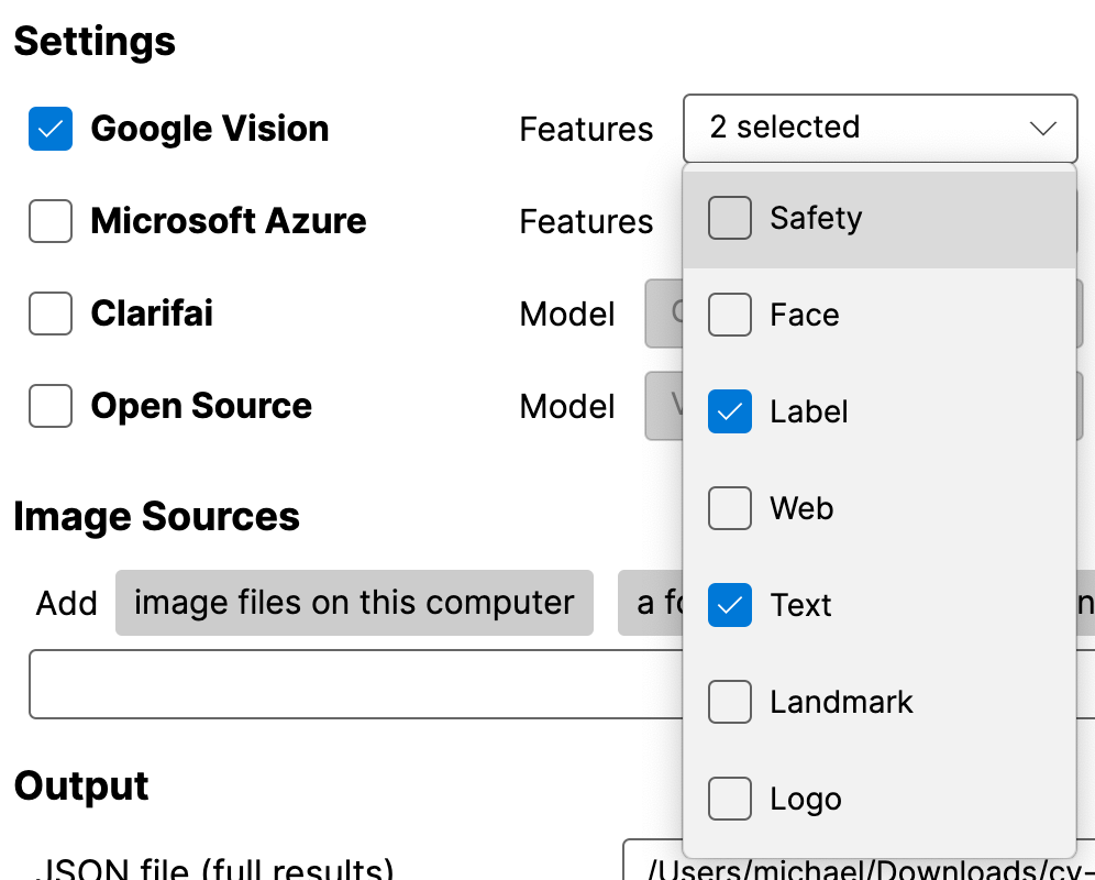
Both methods begin with Memespector (Chao 2023). The software employs commercial APIs like Google Vision AI to classify images with features such as labels or web entities. I recommend selecting Labels and Text initially. The results are stored in two files: a JSON file (which can be quite large) and a CSV file (used in subsequent steps). The CSV format employs a one row per image structure, with multiple labels per image recorded as semicolon-separated values in a single cell. Further details about obtaining a credential file will be provided in class.

Once the API calls succeeded, we can go on and create an image-label-network, or cluster the images based on their labels using k-means.
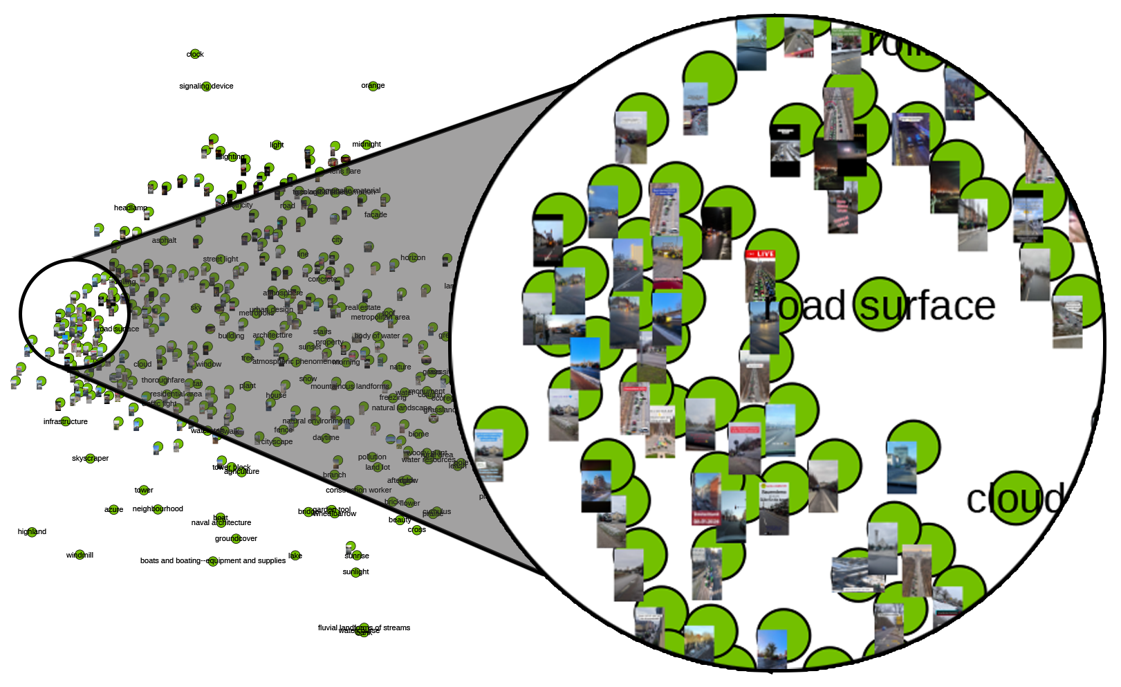
Visual Network Analysis

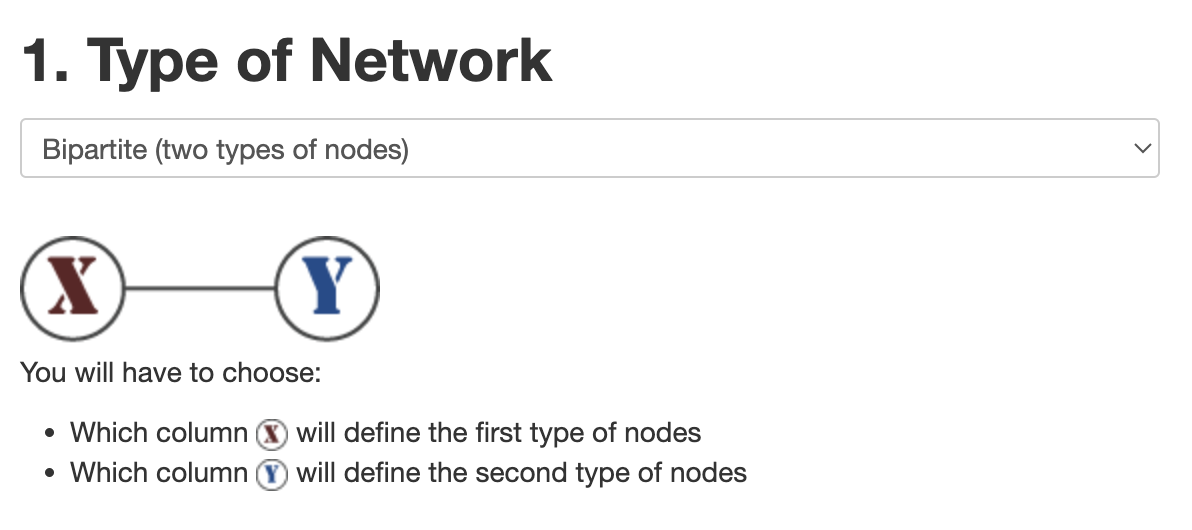
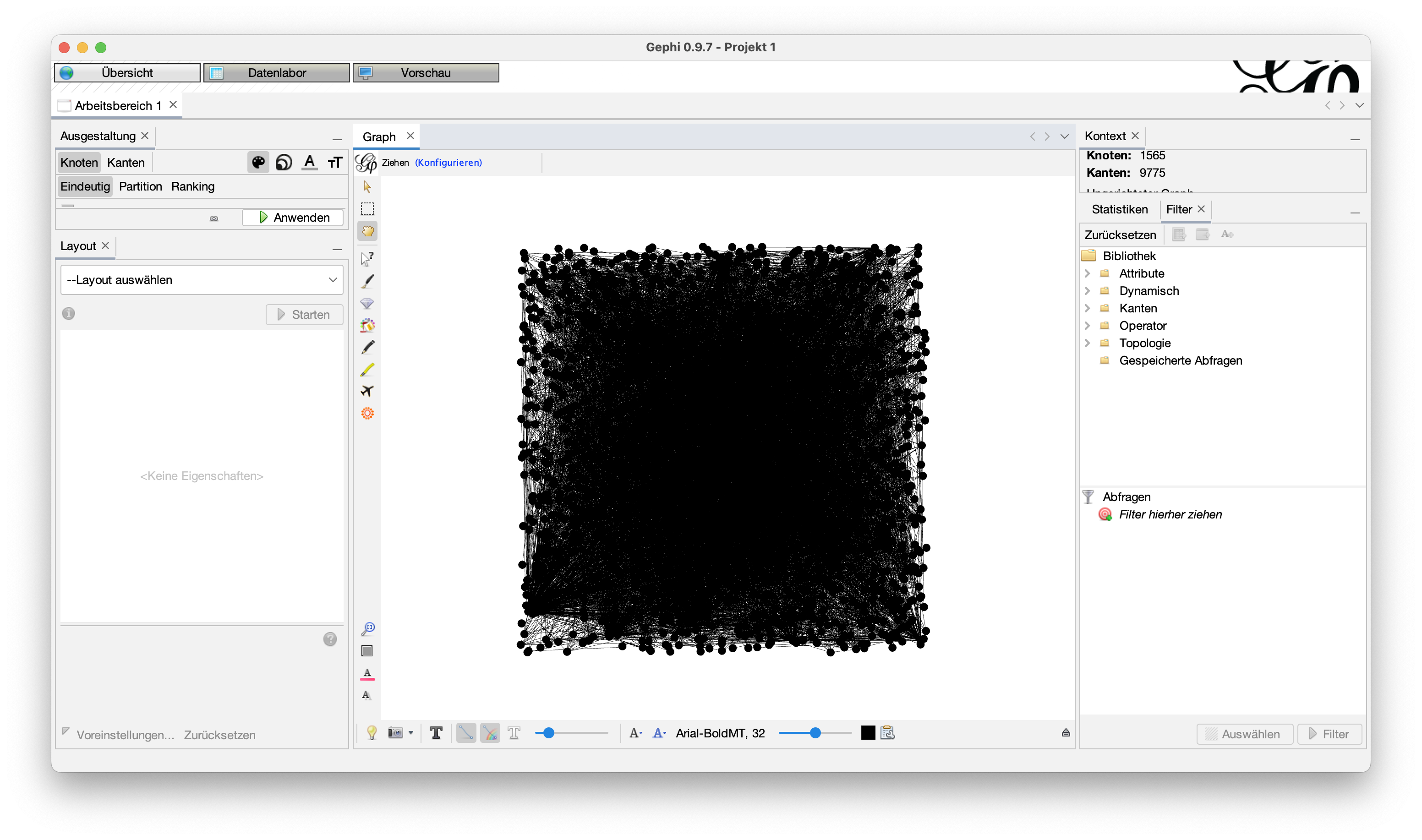
Follow the next steps in order to create your own label-image-network. Gephi is a powerful and complex tool, I omitted a few steps for clarity. Take a look at YouTube tutorials and web tutorials, for more information.
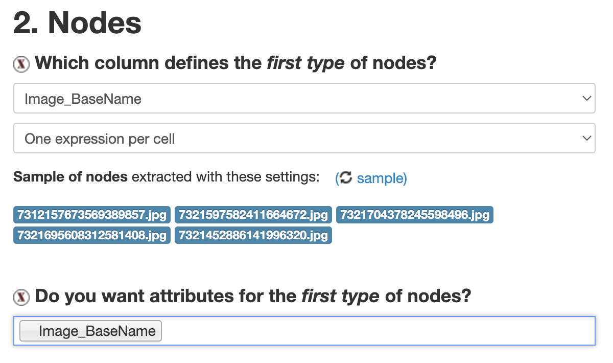
Image_BaseName as the X Node. Additionally, let’s add Image_BaseName again as an attribute, we will use this attribute to display images in Gephi.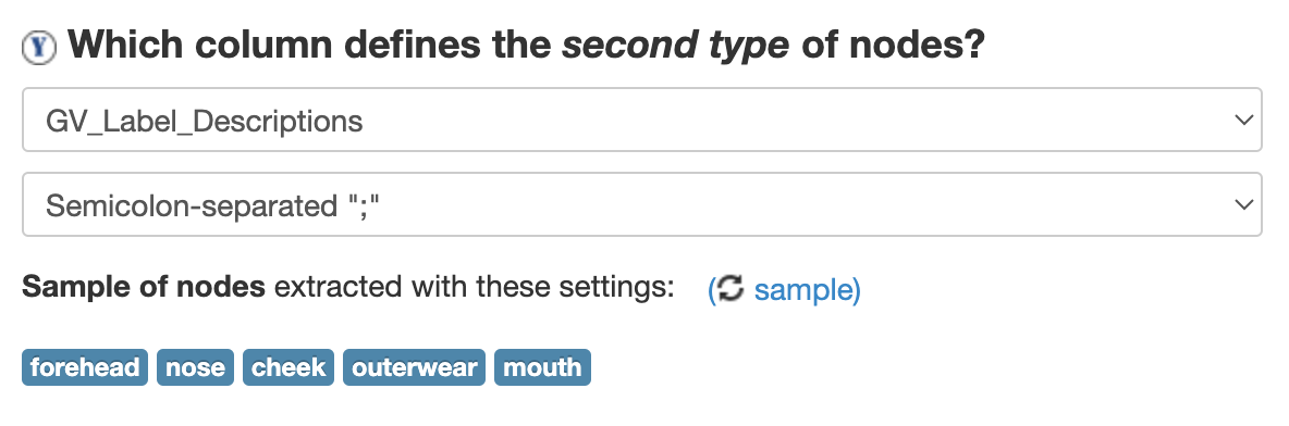
GV_Label_Descriptions column as the second (Y) nodes. Select Semicolon Seperated to split the values in the cell into seperate labels.
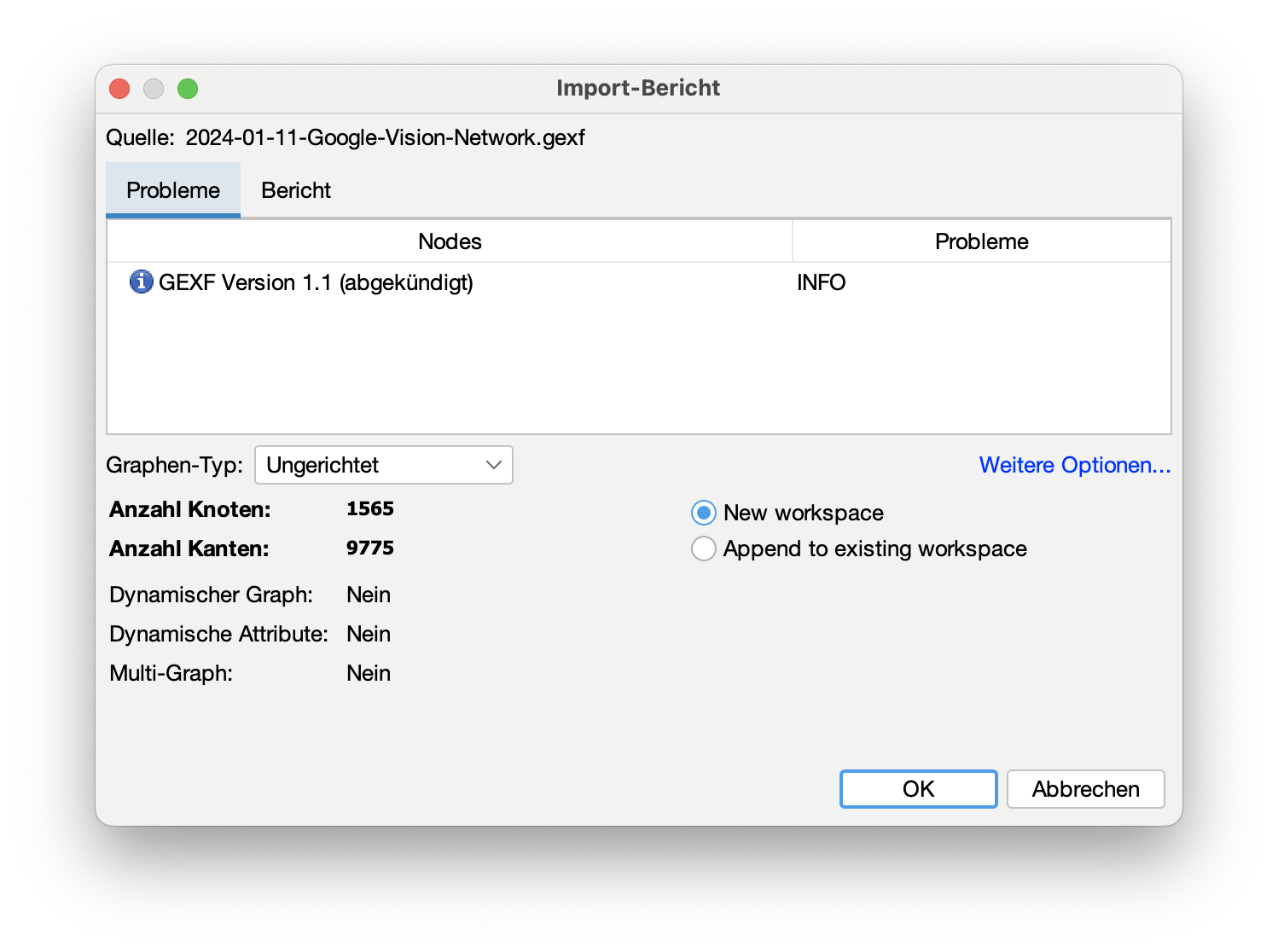
At this stage, after a few seconds of processing, the website should triger the download of a gefxfile. Use Gephi to open this file. Follow these steps:


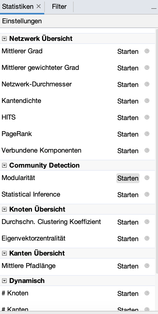

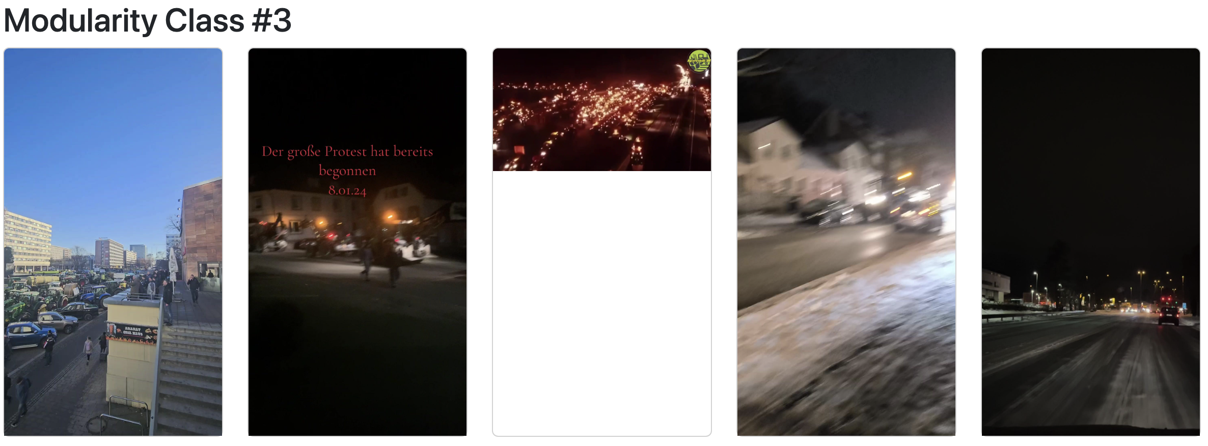
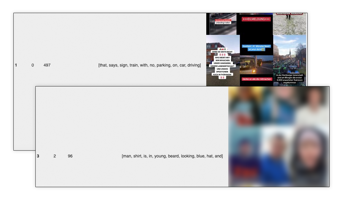
The whole process towards a proper label-image-network contains even more steps, I outsourced them into a document on its own, click here for the missing steps. It’s important to note that working with Gephi, especially when dealing with images, can be demanding in terms of memory usage, and the resulting PDFs are sometimes challenging to handle. To address these issues, I’ve developed a Python script that simplifies the exploration of modularity classes. This script uses a CSV file exported from Gephi to display a selection of images from each class. While this method offers a more manageable way to quickly review samples within each modularity class and assess if we’re on the right track, it’s crucial to acknowledge that we lose certain details in this process. Specifically, this approach doesn’t show the relationships between images and labels, nor does it reveal the spatial distribution of these images within the original network. It’s a trade-off between ease of exploration and the depth of network information,
Follow the next steps to visualize samples from your modularity classes:
Clustering with k-Means
Exploring image corpora using labels or web-entities is just one way of using commercial APIs. Several providers offer models for text detection (OCR), face detection, and more. Below we will take a look at auto-generated image captions – which coincidentally produce text, a data format compatible for exploration and classification using methods established in past sessions. For the k-means approach, we use the image labels and create a matrix with dummy variables: Each labels occupies a column, each image a row, and each cell in the matrix is marked as either True or False. Using this matrix we try to find k-clusters of similar images using the k-means algorithm. First of all I recommend the video below by one of my favorite YouTube channels, for an understanding of the k-means algorithm. Then we take a look at a practical implementation of the algorithm for our visual corpus.
CautionWork-In-Progress
The following notebook is fully functional. It is, however, hardly commented. I will update the notebook and page shortly.
Hands-on k-means
import pandas as pd

# Load the CSV file
memespector_file = "/content/drive/MyDrive/2024-01-09-Bauernproteste/2024-01-11-Google-Vision-All.csv"
df = pd.read_csv(memespector_file)

df = df[['Image_BaseName', 'GV_Label_Descriptions']]

# Splitting the 'GV_Label_Descriptions' into individual labels
split_labels = df['GV_Label_Descriptions'].str.split(';').apply(pd.Series, 1).stack()
split_labels.index = split_labels.index.droplevel(-1)  # to line up with df's index
split_labels.name = 'Label'

# Joining the split labels with the original dataframe
df_split = df.join(split_labels)

# Creating a matrix of True/False values for each label per Image_BaseName
matrix = pd.pivot_table(df_split, index='Image_BaseName', columns='Label', aggfunc=lambda x: True, fill_value=False)

# Resetting the column headers to be the label names only
matrix.columns = [col[1] for col in matrix.columns.values]

# Now 'matrix' has a single level of column headers with only the label namesmatrix| Adaptation | Advertising | Afterglow | Agricultural machinery | Agriculture | Air travel | Aircraft | Airliner | Airplane | Alloy wheel | ... | Vertebrate | Water | Water resources | Wheel | Whiskers | White | Window | Wood | Working animal | World | |
|---|---|---|---|---|---|---|---|---|---|---|---|---|---|---|---|---|---|---|---|---|---|
| Image_BaseName | |||||||||||||||||||||
| 6750551853789891846.jpg | False | False | False | False | False | False | False | False | False | False | ... | False | False | False | False | False | False | False | False | False | False |
| 6750761577349254405.jpg | False | False | False | False | False | False | False | False | False | False | ... | False | False | False | False | False | False | False | False | False | False |
| 6751467034741067014.jpg | False | False | False | False | True | False | False | False | False | False | ... | False | False | False | False | False | False | False | False | False | False |
| 6763591353164254469.jpg | False | False | False | False | False | False | False | False | False | False | ... | False | False | False | False | False | False | False | False | False | False |
| 6766552734108749062.jpg | False | False | False | False | False | False | False | False | False | False | ... | False | False | False | False | False | False | False | False | False | False |
| ... | ... | ... | ... | ... | ... | ... | ... | ... | ... | ... | ... | ... | ... | ... | ... | ... | ... | ... | ... | ... | ... |
| 7321800737606896928.jpg | False | False | False | False | False | False | False | False | False | False | ... | False | False | False | False | False | False | False | False | False | False |
| 7321804342179204384.jpg | False | False | False | False | False | False | False | False | False | False | ... | False | False | False | False | False | False | False | False | False | False |
| 7321804909290999045.jpg | False | False | False | False | False | False | False | False | False | False | ... | False | False | False | True | False | False | False | False | False | False |
| 7321806774967815457.jpg | True | False | False | False | False | False | False | False | False | False | ... | False | False | False | False | False | False | False | False | False | False |
| 7321806890906701089.jpg | False | False | False | False | False | False | False | False | False | False | ... | False | False | False | False | False | False | False | False | False | False |
982 rows × 681 columns
from sklearn.decomposition import PCA
from sklearn.cluster import KMeans
import matplotlib.pyplot as plt
import numpy as np

# Ensuring that 'Image_BaseName' is not part of the matrix to apply PCA
image_base_names = matrix.index  # Saving the image base names for later use
label_matrix = matrix.values  # Convert to numpy array for PCA

# Dimensionality reduction using PCA
# Considering a variance ratio of 0.95 to determine the number of components
pca = PCA(n_components=0.95)
matrix_reduced = pca.fit_transform(label_matrix)

# If needed, you can create a DataFrame from the PCA-reduced matrix and reattach the 'Image_BaseName' column
matrix_reduced_df = pd.DataFrame(matrix_reduced, index=image_base_names)matrix_reduced_df| 0 | 1 | 2 | 3 | 4 | 5 | 6 | 7 | 8 | 9 | ... | 232 | 233 | 234 | 235 | 236 | 237 | 238 | 239 | 240 | 241 | |
|---|---|---|---|---|---|---|---|---|---|---|---|---|---|---|---|---|---|---|---|---|---|
| Image_BaseName | |||||||||||||||||||||
| 6750551853789891846.jpg | 1.392793 | -0.851573 | -0.225060 | -0.630954 | 0.345822 | -0.313126 | 0.376667 | 0.370456 | -0.012519 | -0.898472 | ... | -0.007803 | 0.022912 | -0.002782 | 0.019272 | -0.005465 | -0.005129 | 0.011833 | 0.000200 | 0.006499 | 0.010995 |
| 6750761577349254405.jpg | -1.045212 | 0.139963 | -0.396712 | 0.505531 | -0.186165 | 0.278001 | 0.860551 | -0.387782 | -0.041959 | 0.146992 | ... | 0.020865 | 0.027422 | 0.064993 | 0.046791 | 0.042511 | -0.040843 | -0.091713 | -0.064683 | 0.043392 | -0.045372 |
| 6751467034741067014.jpg | 0.364738 | 0.089808 | 0.603463 | 0.717136 | 0.084382 | 0.130516 | 0.835040 | 0.056190 | -0.175465 | -0.551632 | ... | -0.009497 | 0.144801 | -0.020713 | 0.035502 | -0.085562 | -0.169911 | 0.083582 | 0.045916 | -0.123521 | 0.032273 |
| 6763591353164254469.jpg | 0.657532 | -0.007257 | -0.226448 | -0.142833 | -0.615043 | -0.208217 | -0.082478 | 0.181550 | 0.899774 | 0.462160 | ... | -0.025889 | 0.006257 | 0.060421 | 0.028564 | 0.045773 | 0.000179 | 0.003499 | 0.027838 | 0.007171 | -0.051516 |
| 6766552734108749062.jpg | 1.638604 | -0.418596 | -0.178993 | -0.522654 | 0.663303 | -0.186928 | 1.000894 | -0.307874 | -0.172688 | 0.336597 | ... | -0.009052 | -0.002043 | 0.007575 | -0.031553 | 0.007831 | -0.005779 | -0.023599 | -0.021165 | -0.000496 | -0.006467 |
| ... | ... | ... | ... | ... | ... | ... | ... | ... | ... | ... | ... | ... | ... | ... | ... | ... | ... | ... | ... | ... | ... |
| 7321800737606896928.jpg | -0.698156 | 0.191274 | -0.529836 | 0.047008 | 0.862388 | -0.111187 | -0.390502 | -0.089231 | 0.144091 | 0.326504 | ... | -0.015025 | -0.068188 | -0.023787 | 0.009343 | 0.004624 | 0.001396 | 0.097441 | 0.145987 | -0.102992 | 0.110626 |
| 7321804342179204384.jpg | 0.032051 | 0.048450 | 0.454149 | -0.012114 | 0.395014 | 0.128612 | 0.042362 | 1.019634 | -0.367217 | 1.025644 | ... | -0.002146 | -0.042328 | 0.114229 | -0.066740 | -0.051395 | -0.021397 | 0.012134 | 0.046365 | -0.005712 | 0.036329 |
| 7321804909290999045.jpg | 1.005015 | 0.923683 | 0.371054 | 0.533427 | 0.356759 | 0.813597 | 0.087288 | -0.289707 | 0.377865 | 1.242866 | ... | 0.005721 | 0.000672 | 0.021087 | 0.020260 | 0.037709 | 0.000290 | 0.015725 | 0.013237 | 0.018040 | -0.002060 |
| 7321806774967815457.jpg | -0.597974 | 0.855850 | -0.262498 | -0.214283 | -0.731812 | -0.209626 | -0.179683 | 0.529353 | -0.239506 | 0.048401 | ... | -0.012399 | 0.023383 | -0.073488 | 0.063523 | 0.013320 | 0.020351 | -0.033865 | 0.029809 | -0.080413 | -0.074329 |
| 7321806890906701089.jpg | -0.042383 | -0.138050 | 0.075564 | -0.396196 | 0.056236 | 0.612394 | -0.272538 | -0.230238 | -0.379339 | -0.668773 | ... | -0.106623 | -0.214393 | 0.209117 | 0.021869 | 0.220278 | 0.070092 | -0.198979 | 0.140981 | -0.004653 | -0.070667 |
982 rows × 242 columns
# Elbow method to determine optimal number of clusters
inertia = []
range_values = range(1, 20)  # Checking for 1 to 10 clusters

for i in range_values:
    kmeans = KMeans(n_clusters=i, n_init=10, random_state=0)
    kmeans.fit(matrix_reduced_df)
    inertia.append(kmeans.inertia_)

# Plotting the Elbow Curve
plt.figure(figsize=(10, 6))
plt.plot(range_values, inertia, marker='o')
plt.title('Elbow Method')
plt.xlabel('Number of clusters')
plt.ylabel('Inertia')
plt.show()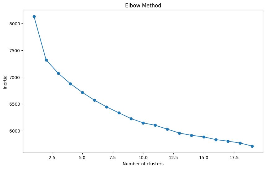
from sklearn.cluster import KMeans
from sklearn.metrics import silhouette_score
import matplotlib.pyplot as plt

# Define the range of clusters to try
range_values = range(2, 20)

silhouette_scores = []

# Perform k-means clustering and compute silhouette scores
for i in range_values:
    try:
        kmeans = KMeans(n_clusters=i, n_init=10, random_state=0)
        kmeans.fit(matrix_reduced_df)
        score = silhouette_score(matrix_reduced_df, kmeans.labels_)
        silhouette_scores.append(score)
    except Exception as e:
        print(f"An error occurred with {i} clusters: {e}")

# Plotting the Silhouette Scores
with plt.style.context('seaborn-whitegrid'):
    plt.figure(figsize=(10, 6))
    plt.plot(range_values, silhouette_scores, marker='o')
    plt.title('Silhouette Method')
    plt.xlabel('Number of clusters')
    plt.ylabel('Silhouette Score')
    plt.show()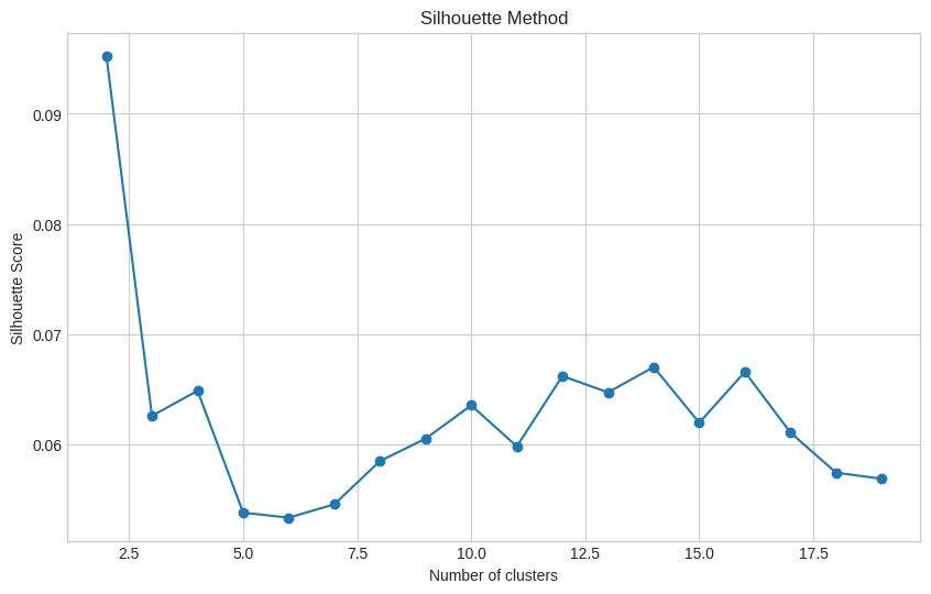
# Final k-means clustering using n clusters
kmeans_final = KMeans(n_clusters=11, n_init=10, random_state=0)
clusters = kmeans_final.fit_predict(matrix_reduced)

# Adding the cluster information back to the original dataframe
matrix['Cluster'] = clusters
# Displaying the first few rows of the dataframe with cluster information
matrix.head()| Adaptation | Advertising | Afterglow | Agricultural machinery | Agriculture | Air travel | Aircraft | Airliner | Airplane | Alloy wheel | ... | Water | Water resources | Wheel | Whiskers | White | Window | Wood | Working animal | World | Cluster | |
|---|---|---|---|---|---|---|---|---|---|---|---|---|---|---|---|---|---|---|---|---|---|
| Image_BaseName | |||||||||||||||||||||
| 6750551853789891846.jpg | False | False | False | False | False | False | False | False | False | False | ... | False | False | False | False | False | False | False | False | False | 8 |
| 6750761577349254405.jpg | False | False | False | False | False | False | False | False | False | False | ... | False | False | False | False | False | False | False | False | False | 2 |
| 6751467034741067014.jpg | False | False | False | False | True | False | False | False | False | False | ... | False | False | False | False | False | False | False | False | False | 6 |
| 6763591353164254469.jpg | False | False | False | False | False | False | False | False | False | False | ... | False | False | False | False | False | False | False | False | False | 0 |
| 6766552734108749062.jpg | False | False | False | False | False | False | False | False | False | False | ... | False | False | False | False | False | False | False | False | False | 8 |
5 rows × 682 columns
!unzip /content/drive/MyDrive/2024-01-09-Bauernproteste/2024-01-09-Images-Clean.zip# Display the result. See linked notebook for code.BERTopic
Summary
I introduced several unsupervised approaches for exploring visual corpora. The first part of this article introduced commercial computer vision APIs as a source for labels describing the content of images, the second part derived the knowledge of image content by generating image captions. Using these captions we fit a topic model, that helped to cluster the images into classes. Overall, the approaches result in two or more groups of images, that show similarities. What makes an image similar, is based on the model we apply. PicArrange, for example, uses colours, while other approaches focus on detected objects and labels describing the content of images. These groups need human exploration in order to make sense of them. The exploration techniques can be useful for a first exploration of your visual corpus. In the next session we go one step further, we will classify images based on their content using different approaches, like CLIP and GPT-4.
References
Chao, Jason. 2023. “Memespector-GUI: Graphical User Interface Client for Computer Vision APIs.” https://doi.org/10.5281/zenodo.7704877.
Omena, Janna Joceli, Pilipets Elena, Beatrice Gobbo, and Chao Jason. 2021. “The Potentials of Google Vision API-based Networks to Study Natively Digital Images.” Diseña, no. 19 (September): 1–1. https://doi.org/10.7764/disena.19.Article.1.
Sánchez-Querubı́n, Natalia, Shuaishuai Wang, Briar Dickey, and Andrea Benedetti. 2023. “Political TikTok: Playful performance, ambivalent critique and event-commentary.” In The Propagation of Misinformation in Social Media, edited by Richard Rogers, 187–206. A Cross-Platform Analysis. Amsterdam University Press. https://doi.org/10.2307/jj.1231864.12.
Reuse
Citation
BibTeX citation:
@online{achmann-denkler2024,
  author = {Achmann-Denkler, Michael},
  title = {Visual {Exploration}},
  date = {2024-01-15},
  url = {https://social-media-lab.net/image-analysis/exploration.html},
  doi = {10.5281/zenodo.10039756},
  langid = {en}
}
For attribution, please cite this work as:
Achmann-Denkler, Michael. 2024. “Visual Exploration.”
January 15, 2024. https://doi.org/10.5281/zenodo.10039756.