Text as Data

The analysis of texutal data has a long tradition under the term Natural Language Processing (NLP). As noted by Bengfort, Bilbro, and Ojeda (2018), “Language is unstructured data that has been produced by people to be understood by other people”. This characterization of language as unstructured data highlights its contrast with structured or semi-structured data. Unlike structured data, which is organized in a way that computers can easily parse and analyze, unstructured data like language requires more complex methods to be processed and understood. In the context of e.g. Instagram, CrowdTangle exports contain structured data columns such as ‘User Name’, ‘Like Count’, or ‘Comment Count’. These pieces of data are quantifiable and can be easily sorted, filtered, or counted, e.g. using tools like Excel or Python’s pandas library. For instance, we can quickly determine the most active users by counting the number of rows associated with each username. In contrast, unstructured data is not organized in a predefined manner and is typically more challenging to process and analyze. The ‘Description’ column in our dataset, which contains the captions of Instagram posts, is a prime example of unstructured data. These captions, composed of paragraphs or sentences, require different analytical approaches to extract meaningful insights. Unlike structured data, we cannot simply count or sort these texts in a straightforward manner. In our context, we often refer to the collection of texts we analyze as a “Corpus”. Each individual piece of text is called a “Document”. Each document can be broken down into smaller units known as “features”. Features can be words, phrases, or even patterns of words, which we then use to quantify and analyze the text (compare p. 230 Haim 2023). For the goal of our research seminar, we can follow the three technical perspectives inspired by Haim (2023): 1. Frequency Analysis, 2. Contextual Analysis, and 3. Content Analysis.

Outline

1. Data Structure and Preprocessing
   We examine the data structure, import data from Zeeschuimer, and create the first metadata table. This provides an organized overview of the corpus, laying the foundation for the next steps.

2. Preprocessing for Text Extraction
   In this phase, we focus on obtaining OCR text from images and transcriptions from audio content. This ensures that all embedded text in images and videos is converted into machine-readable formats, preparing the data for analysis.

3. Data Exploration
   With the text extracted, we move to exploratory analysis. Here, we conduct frequency analyses and other exploratory techniques to gain insights into the corpus, identifying prominent themes or topics. Tools like GPT and possibly BERTopic may be used for deeper exploration.

4. Classification and Coding
   Finally, we apply classification methods to categorize text into predefined groups or themes, providing a more nuanced, quantitative understanding of the content.

Organizing Data for Social Media Analysis

This section explains how to structure metadata, text, and visual data for effective analysis. My recommendations are just one example of organizing the data, but the key is following a consistent structure across a project. For the present course, adhering to a set data structure is essential for using the example notebooks effectively.

General Data Structure

To analyze Instagram Stories or posts, we organize data into multiple tables, each focusing on a specific content type:

1. Metadata Table: This table contains basic metadata such as story ID, username, and other general attributes. Each story is represented by one row.
2. Text Table: This table stores text content, like OCR results, transcriptions, and captions. Each text entry is assigned a unique Text ID and is linked back to the Story ID to connect it with the metadata.
3. Images Table: This table contains information about images or videos, which are also linked to the Story ID for easy integration across datasets.

To ensure that our data is organized and clean for analysis, we follow the Tidy Data Principles:

1. Each variable forms a column.
2. Each observation forms a row.
3. Each type of observational unit forms a table.

Visualization of the tidy data components, source: R for Data Science.

This structure, inspired by Tidy Data (Wickham 2014), ensures that our data is clean, consistent, and accessible to analyze. In social media data, a post is often treated as an observation,Depending on the content type, such as an album, each image might be treated as a separate observation making it a row in our tables. as a separate observation depending on the content type, such as an album.

Figure 1: An example for mapping multiple rows of text in the Text Table to a single row in the metadata table Story Table

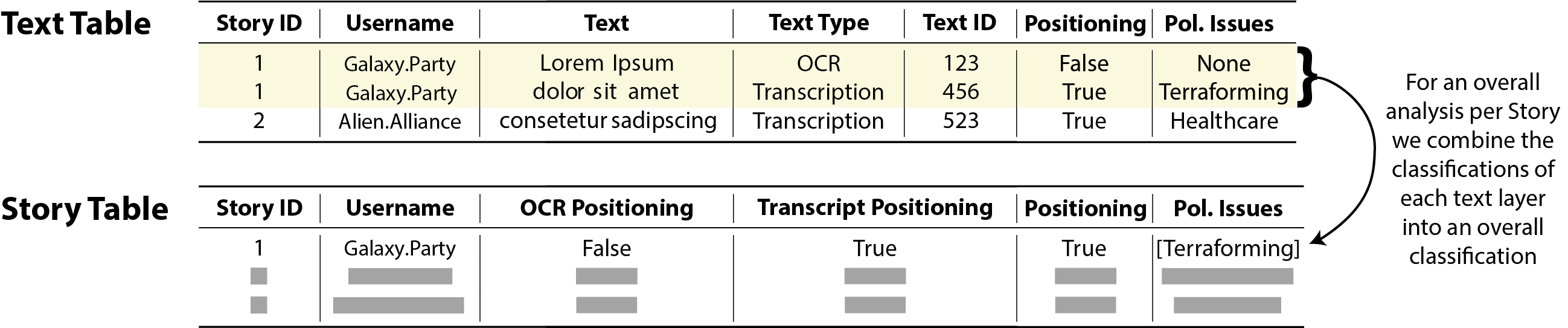
Figure 1 shows how data from different layers, like text and the variables Policy Issues and Positioning, can be aggregated at the story level. Policy Issues is a categorical variable that references different policy topics, while Positioning is a Boolean variable that is True if a given text mentions any policy issues and False otherwise. The figure illustrates the integration process and highlights how various types of information are combined into a cohesive dataset. Note that these variables are just examples—they can change based on the research question. This structure is flexible, allowing adaptation to different research needs.

Decomposing Text and Image Data

The Text Table may include several text types for each story, such as OCR text and transcriptions, each identified by Story ID. Columns in this table typically include:

• Story ID: Links to the main metadata.
• Text Type: Specifies the origin of the text (e.g., OCR, transcription).
• Text ID: A unique identifier for each text entry.
• Other columns like Positioning or Policy Issues can be added depending on the research focus.

We follow a similar approach for images with the Images Table, which contains one row per image. Columns in the Images Table typically include:

• Image ID: A unique identifier for each image.
• Story ID: Links to the main metadata to ensure traceability to the original post.
• Other columns may include attributes like image description or Image Type.

When dealing with more complex data, such as Instagram albums with multiple images per post, we consider each image or video as a separate observation. In such cases, the ID column helps maintain a fixed reference to the original post, allowing us to re-merge the data later with post-level metadata.

Metadata Table and Aggregation

The Metadata Table aggregates data from multiple content layers, summarizing attributes like Positioning and Policy Issues for each post or story. For Boolean variables like Positioning, the overall value is set to True if any text component indicates a position. For categorical variables like Policy Issues, unique values from all components are combined into a list. Depending on your research focus, you might also consider other methods, such as counting occurrences instead of simple aggregation. The flexibility of this approach allows you to adapt the analysis to either story-level or post-level data as needed.

The Zeeschuimer Import Notebook helps create the initial metadata table for posts collected through Zeeschuimer. Similarly, when using Tidal Tales, we can use the CSV downloaded from the extension as our metadata table, and the same applies to the Meta Content Library. However, for the latter, we might need to rename columns to ensure compatibility when using the example notebooks provided on this website.

Note

I updated the Zeeschuimer Import Notebook to handle gallery posts. The new version creates one row per image. Thus, when using the new notebook, we still need to manually create the metadata table. The old Zeeschuimer Import Notebook is still available – it creates one row per post and only downloads one image.

Data Normalization with the Notebook

We use the Zeeschuimer Import Notebook notebook to standardize raw data collected through the Zeeschuimer Plugin, specifically importing the data from Zeeschuimer as jsonl files and transforming them into a pandas DataFrame. While Zeeschuimer and 4CAT provide a good standard data structure, we aim to work with data from multiple sources: Zeeschuimer, Tidal Tales (a Firefox extension for collecting IG stories), Meta Content Library, or TikTok data from Zeeschuimer. The notebook helps convert Zeeschuimer data into the unified structure that we use across all projects, ensuring consistency.

The Zeeschuimer Import Notebook helps us systematically prepare data for analysis:

• Data Import: Imports data from sources like CrowdTangle and 4CAT using tools such as pandas and json.
• Data Sampling: Displays random samples to check accuracy and ensure data correctness at each step.
• Normalization: Converts different text types (e.g., OCR, transcriptions) into standardized DataFrames.
• Media Management: Organizes media files into folders following a consistent structure. For images, the files are saved in images/{username}/{ID}.jpg, and for videos, in videos/{username}/{ID}.mp4. The video cover image is also saved as a file in the case of videos. The notebook also handles gallery posts, saving images with filenames such as {ID}_0.jpg, {ID}_1.jpg, etc.

Note

This page and the referenced notebooks cover the data formats and media files of Zeeschuimer and Tidal Tales. Generally, the information also applies when using other software, like instaloader. To control media file names, it is advisable to use the --filename-pattern command line parameter. This makes mapping JSON metadata to media objects easier. After loading all posts and stories with instaloader, I recommend reading all JSON files in a loop and creating a DataFrame. For more information and code examples, see Data Collection / Posts / Instaloader.

Best Practices for Data Integration

• Consistent Identifiers: Use consistent identifiers like Story ID and Username across all tables to facilitate data merging.
• Unique IDs: Assign unique IDs for each element (e.g., Text ID, Image ID) to make tracking and linking straightforward.
• Organized Directory Structure: Store media files systematically. For images, use images/{username}/{ID}.jpg and for videos, use videos/{username}/{ID}.mp4. In the case of gallery posts, use filenames like {ID}_0.jpg, {ID}_1.jpg, etc., and reference these paths in your tables for easy access.
• Data Integration: Use tools like pandas to merge tables based on shared identifiers, enabling a complete view of each story or post.
• Backup Strategy: When working with experimental code, keep backups of your data file and avoid overwriting the original file until you are confident in the results.

By following these guidelines, you will keep your data well-organized, reproducible, and ready for detailed analysis, minimizing complexity and enhancing your insights’ quality.

More Resources

Python & Computational Social Sciences

• Python for Computational Social Science and Digital Humanities (YouTube)
• Introduction to Computational Social Science methods with Python (Online)
• Introduction to Data Science: A Python Approach to Concepts, Techniques and Applications (E-Book)
• R for Data Science (2nd edition) – not Python, but the principles can easily be migrated to pandas.

Python & NLP

• Natural Language Processing (Notebook, GESIS CSS)
• Word Frequencies (Online)
• Introduction Jupyter Notebooks (Online)
• Konchady (2016): Text Mining Application Programming (Somewhat older, still an interesting reading for the basics of computational corpus analysis)

References

Bengfort, Benjamin, Rebecca Bilbro, and Tony Ojeda. 2018. Applied Text Analysis with Python: Enabling Language-Aware Data Products with Machine Learning. “O’Reilly Media, Inc.”

Haim, Mario. 2023. Computational Communication Science: Eine Einführung. Springer Fachmedien Wiesbaden.

Wickham, Hadley. 2014. “Tidy Data.” Journal of Statistical Software, Articles 59 (10): 1–23. https://doi.org/10.18637/jss.v059.i10.