
function drawCodingPlot(coder1, coder2) {
    const svgWidth = coder1.length * 10 + 100; // Adjust the width based on the number of items and space for labels
    const svgHeight = 50; // Fixed height, two rows
    const svg = d3.create("svg")
                  .attr("width", svgWidth)
                  .attr("height", svgHeight);

    // Adding labels for Coders
    svg.append("text")
       .attr("x", 40)
       .attr("y", 20)
       .text("Coder 1")
       .attr("font-size", "10px")
       .attr("text-anchor", "end");

    svg.append("text")
       .attr("x", 40)
       .attr("y", 40)
       .text("Coder 2")
       .attr("font-size", "10px")
       .attr("text-anchor", "end");

    // Drawing circles for codings
    coder1.forEach((code, index) => {
        svg.append("circle")
           .attr("cx", 60 + 10 * index)
           .attr("cy", 15)
           .attr("r", 4)
           .style("fill", code === 1 ? "black" : "none")
           .style("stroke", "black");
    });

    coder2.forEach((code, index) => {
        svg.append("circle")
           .attr("cx", 60 + 10 * index)
           .attr("cy", 35)
           .attr("r", 4)
           .style("fill", code === 1 ? "black" : "none")
           .style("stroke", "black");
    });

    return svg.node();
}


// Function to generate controlled codings
function generateControlledCoding(nItems, disagreementRate) {
    let coder1 = Array.from({length: nItems}, () => Math.random() < 0.5 ? 0 : 1);
    let coder2 = [...coder1];
    disagreementRate = disagreementRate / 100
    let nDisagreements = Math.floor(nItems * disagreementRate);
    for (let i = 0; i < nDisagreements; i++) {
        let index = Math.floor(Math.random() * nItems);
        coder2[index] = 1 - coder2[index];
    }
    return [coder1, coder2];
}

// Function to calculate Cohen's Kappa
function calculateCohensKappa(coder1, coder2) {
    let totalItems = coder1.length;
    let agree = 0;
    let coder1Yes = 0;
    let coder2Yes = 0;

    for (let i = 0; i < totalItems; i++) {
        if (coder1[i] === coder2[i]) {
            agree++;
        }
        if (coder1[i] === 1) {
            coder1Yes++;
        }
        if (coder2[i] === 1) {
            coder2Yes++;
        }
    }

    let Po = agree / totalItems;
    let Pe = (coder1Yes / totalItems) * (coder2Yes / totalItems) +
             ((totalItems - coder1Yes) / totalItems) * ((totalItems - coder2Yes) / totalItems);

    return (Po - Pe) / (1 - Pe);
}

viewof disagreement_rate = Inputs.range([0, 100], {step: 1.0, value: 10, label: "Disagreement"})
viewof nItems = Inputs.range([11, 65], {step: 1.0, value: 65.0, label: "n"})

// Main calculation and display
{
    const [coder1, coder2] = generateControlledCoding(nItems, disagreement_rate);
    const kappa = calculateCohensKappa(coder1, coder2);

    // Draw the coding plot
    const codingPlot = drawCodingPlot(coder1, coder2);

    return html`<div>Cohen's Kappa: ${kappa.toFixed(2)}</div>
                  <div>${codingPlot}</div>`;
}Agreement & Evaluation
The previous chapter focused on the creation of a Ground Truth dataset using human annotations. In this chapter we pick up on the annotated data and will first assess the quality of the annotations before adopting them as a gold standard. The integrity of the dataset directly influences the validity of our model evaluations. Klie, Castilho, and Gurevych (2024) emphasize that proper quality management, including interrater agreement, manual inspection, and an iterative annotation processes, is vital for mitigating such issues and producing datasets suitable for real-world applications.
To this end, we take a look at two interrater agreement measures: Cohen’s Kappa and Krippendorff’s Alpha. These metrics are important for quantifying the level of agreement among annotators. Once we established the quality of our annotations, we will use them as ground truth. In our context there are two use cases for the ground truth dataset: When training or fine-tuning our own model, we need a training for our model to learn from. Additionally, we always–for training our model as well as using LLMs–need an evaluation dataset to determine how well our computational approach performs when applied to real-world data. The performance of machine learning models is typically assessed using a variety of metrics, each offering a different perspective on the model’s effectiveness. In this chapter, we will take a look at four fundamental metrics: Accuracy, Precision, Recall, and F1 Score.
In the first part of the chapter we will take a look at interrater agreements and machine learning evaluation measures. In the application part I provide the notebooks to:
- Import Label Studio Annotations
- Calculate the interrater measures
- Derive the gold standard from the annotations
- Calculate the evaluation metrics for your model based on the gold standard.
Finally, the optimization part of this page provides an outlook for how to use the evaluation metrics in order to tune your classification prompt.
ImportantUpdate 2024
- Link to Notebook.
- Updated the notebook to handle both, single annotation projects (from the enterprise version of Label Studio), and multiple annotation projects (when using the Open Source version).
Interrater Agreement
Cohen’s \(\kappa\)
is a widely used statistic for measuring the agreement between two annotators, taking into account the agreement occurring by chance. This metric is particularly valuable when dealing with categorical data, as is often the case in text annotations. Cohen’s Kappa provides a more robust measure than simple percent agreement calculation because it considers the possibility of the agreement occurring randomly. The kappa score can range from -1 (complete disagreement) to 1 (complete agreement), with 0 indicating the level of agreement that can be expected from random chance.
The definition of \(\kappa\) is:
\(\kappa \equiv \frac{p_o - p_e}{1 - p_e} = 1- \frac{1 - p_o}{1 - p_e}\)
“where \(p_{0}\) is the relative observed agreement among raters, and \(p_{e}\) is the hypothetical probability of chance agreement, using the observed data to calculate the probabilities of each observer randomly seeing each category.” (Source: Wikipedia)
Using python we can easily calculate Cohen’s Kappa:
from sklearn.metrics import cohen_kappa_score

# Example annotations from two annotators
annotator1 = [1, 2, 3, 4, 5]
annotator2 = [2, 2, 3, 4, 4]

kappa = cohen_kappa_score(annotator1, annotator2)
print(f"Cohen's Kappa: {kappa}")
Krippendorff’s \(\alpha\)
While Cohen’s Kappa is ideal for pairwise annotation evaluation, Krippendorff’s Alpha is used when there are more than two annotators. This metric is versatile as it can handle various types of data, including nominal, ordinal, interval, or ratio-scaled. Krippendorff’s Alpha assesses the agreement among multiple annotators, accounting for the possibility of chance agreement. Its value also ranges from -1 to 1, with higher values indicating better reliability and 0 representing agreement equivalent to chance.
The definition of \(\alpha\) is:
\(\alpha = 1-\frac{D_o}{D_e}\)
“where \(D_o\) is the disagreement observed and \(D_e\) is the disagreement expected by chance.” (Source: Wikipedia)
Static Example
Calculating the Krippendorff Alpha is more complex than Cohen’s kappa. The example below is static, use the code below to calculate Krippendorff’s Alpha in your Jupyter Notebook.
n: 65
Disagreement: 10%
Krippendorff's Alpha: 0.8164136622390892
In order to calculate Krippendorff’s Alpha using python we need to install the krippendorff package: pip install krippendorff. Calculating the \(\alpha\) value using python is straightforward – as long as the codings are provided as integers.
import krippendorff
import numpy as np

# Example annotations from three annotators
data = np.array([
    [1, 2, 3, 4, 5],
    [2, 2, 3, 4, 4],
    [1, 2, 4, 4, 5]
])

alpha = krippendorff.alpha(data)
print(f"Krippendorff's Alpha: {alpha}")
In case of e.g. strings (categorical data), we need to encode the values first:
data_categorical = [
    ["yes", "no", "yes", "maybe", "no"],
    ["no", "no", "yes", "maybe", "maybe"],
    ["yes", "no", "maybe", "maybe", "no"]
]

# Convert categorical data to numerical format
label_encoding = {"yes": 0, "no": 1, "maybe": 2}
data_encoded = np.array([[label_encoding.get(item, np.nan) for item in row] for row in data_categorical])

alpha = krippendorff.alpha(data_encoded)
print(f"Krippendorff's Alpha: {alpha}")
Machine Learning Evaluation Metrics
After establishing the reliability of our annotations, we now turn our attention to evaluating the performance of machine learning models using these validated datasets. This is crucial for understanding how well our computational approaches are performing in real-world scenarios. In this segment, we discuss four evaluation metrics: Accuracy, Precision, Recall, and F1 Score.
Warning
This subchapter scratches the surface. Recommended reading: e.g. Haim (2023) pp. 246–252, or machine learning textbooks. Parts of this section have been generated using ChatGPT (e.g. examples).
Understanding Confusion Matrix Components
Before diving into the metrics, it’s important to understand the components of a confusion matrix: True Positives, True Negatives, False Positives, and False Negatives. Here’s a brief explanation of each:
- True Positives (TP): These are cases where the model correctly predicts the positive class.
- True Negatives (TN): These are cases where the model correctly predicts the negative class.
- False Positives (FP): These are cases where the model incorrectly predicts the positive class (also known as a “Type I error”).
- False Negatives (FN): These are cases where the model incorrectly predicts the negative class (also known as a “Type II error”).
The following table summarizes these concepts:
| Actual Positive | Actual Negative | |
|---|---|---|
| Predicted Positive | True Positives (TP) | False Positives (FP) |
| Predicted Negative | False Negatives (FN) | True Negatives (TN) |
Example Scenario:
Consider a social media sentiment analysis model that classifies posts as either “Positive” or “Negative.” In this context:
- A True Positive would be a post that is actually positive and the model also predicts it as positive.
- A True Negative would be a post that is actually negative and the model also predicts it as negative.
- A False Positive would occur if the model incorrectly classifies a negative post as positive.
- A False Negative would occur if the model incorrectly classifies a positive post as negative.
Understanding these components is key to interpreting the subsequent metrics which are derived from the values in the confusion matrix. These metrics – Accuracy, Precision, Recall, and F1 Score – are applicable to both binary (as showcased above) and multi-class classification problems. The concept of True / False Positives / Negatives remains the same, but for multi-class scenarios, they are computed per class and then averaged to provide overall model performance.
Accuracy: A General Overview
Accuracy is the simplest and most straightforward metric. It represents the ratio of correctly predicted observations (both true positives and true negatives) to the total observations in the dataset.
\(\text{Accuracy} = \frac{\text{True Positives (TP)} + \text{True Negatives (TN)}}{\text{Total Observations}}\)
Accuracy can be misleading, particularly in datasets where class distributions are imbalanced. In such cases, a model might appear to perform well simply by favoring the majority class, while failing to accurately predict the minority class.
Precision: Measuring Exactness
Precision reflects the accuracy of positive predictions. It shows how many of the items identified as positive are actually positive. This metric is vital when the costs of false positives are high.
\(\text{Precision} = \frac{\text{True Positives (TP)}}{\text{True Positives (TP)} + \text{False Positives (FP)}}\)
High precision indicates a low rate of false positives, which is essential in scenarios where false alarms are costly or dangerous.
Recall: Assessing Completeness
Recall, or sensitivity, measures the model’s ability to identify all relevant instances. In other words, it shows how many of the actual positive cases were correctly identified by the model.
\(\text{Recall} = \frac{\text{True Positives (TP)}}{\text{True Positives (TP)} + \text{False Negatives (FN)}}\)
High recall is crucial in situations where missing a positive instance has severe implications, like in medical diagnoses.
F1 Score: Harmonizing Precision and Recall
The F1 Score is the harmonic mean of Precision and Recall, offering a balance between the two. It is particularly useful when you need a single metric to reflect a model’s performance, especially in cases of uneven class distribution.
\(\text{F}_{1} = 2 \times \frac{\text{Precision} \times \text{Recall}}{\text{Precision} + \text{Recall}}\)
A high F1 Score suggests a robust model with a good balance between precision and recall.
Warning
While a high F1 Score is often seen as indicative of a model’s effectiveness, it’s important to approach this metric with caution. The F1 Score, being a harmonic mean of precision and recall, may not comprehensively represent the performance nuances in certain contexts, especially in imbalanced datasets where either false positives or false negatives are more consequential. Refer to the criticism section in the Wikipedia article on F1 Score or e.g. the paper “Performance Evaluation in Machine Learning: The Good, the Bad, the Ugly, and the Way Forward” by Flach (2019).
Evaluation Multi-Class Models
When evaluating multi-class classification models, we often need to summarize the performance across all classes. This is where macro, micro, and weighted averages come into play. Each of these averages provides a different perspective on the model’s performance and is useful in various scenarios.
- The macro average is calculated by taking the mean of the metrics, such as precision, recall, or F1 score, computed independently for each class. It treats all classes equally, giving equal weight to the performance on each class regardless of its frequency.
- The micro average aggregates the contributions of all classes to compute the average metric. It calculates the metrics globally by counting the total true positives, false negatives, and false positives.
- The weighted average calculates each metric for each class like the macro average but takes the size of the class into consideration when averaging. Therefore, it accounts for class imbalance by giving more weight to the metrics of larger classes.
Choosing the Right Average:
- Use Macro Averages when you are dealing with imbalanced datasets or when you consider each class equally important.
- Use Weighted Averages when each class’s importance is proportional to its size and you want to weight your metric by class distribution.
- Use Micro Averages if you have a balanced dataset and want an easily understandable metric for overall performance regardless of the class.
Reporting
When presenting the results of a machine learning model’s performance, especially in the context of academic research, the method of reporting is critical. A confusion matrix, such as the one shown below, is a great visualization tool for both, single- and multi-class classification tasks, like in the example below, where I experimented with face recognition on social media images.
The confusion matrix visualizes the model’s predictions in comparison to the true labels, allowing for an immediate grasp of the model’s performance across various classes. It also succinctly illustrates the number of false positives, false negatives, true positives, and true negatives, providing a clear visual summary of the model’s predictive power.
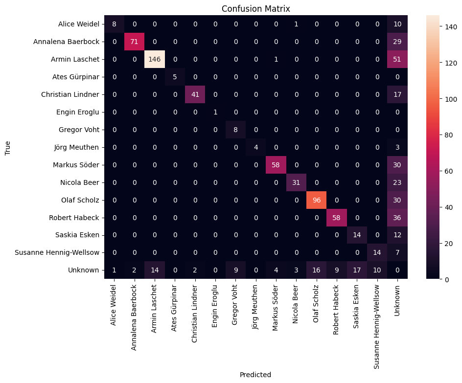
The color intensity in each cell corresponds to the count, with darker cells indicating higher numbers. This visual gradation allows for quick identification of which classes are being predicted accurately and which are not.
However, a confusion matrix is just one of the tools at our disposal for reporting performance metrics. In many cases, supplementing the confusion matrix with additional tables that break down key metrics like accuracy, precision, recall, and F1 score can provide a more nuanced understanding. For example, a table could list each class along with the corresponding precision and recall, giving a clear indication of where the model excels and where it may require further tuning.
| Class/Category | Accuracy | Precision | Recall | F1 Score |
|---|---|---|---|---|
| Alice Weidel | 0.90 | 0.88 | 0.92 | 0.90 |
| Annalena Baerbock | 0.93 | 0.94 | 0.89 | 0.91 |
| Armin Laschet | 0.85 | 0.83 | 0.88 | 0.85 |
| … | … | … | … | … |
| Macro Average | 0.92 | 0.91 | 0.90 | 0.91 |
| Micro Average | 0.92 | 0.92 | 0.92 | 0.92 |
| Weighted Average | 0.93 | 0.92 | 0.93 | 0.93 |
In our projects reports, we will also include such tables and graphs to comprehensively present the model’s performance, ensuring that we communicate the most detailed insights to our readers.
Annotation Export
In this section I will guide you step-by-step through the export of annotations from label studio, the calculation of interrater agreements, the process of deriving the gold standard, and finally the evaluation of your model (prompt).
We are going to use some sample data from one of my projects. The goal was to classify three content variables for social media texts. The content was either from captions, OCR, or transcribed audio. Three annotators were tasked to code each variable.
Exporting the annotations is straightforward: On the dashboard of your project, click “Export”:

Next, choose “Create New Snapshot” (Step 1). When creating the snapshot we may keep the original settings, click “Create Snapshot”. The application takes you back to the previous screen. Now we’re ready to click “Download” (Step 3). Your browser starts downloading a JSON file. Depending on the amount of annotations, it may take a while to open the file.


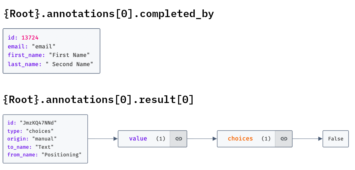
The JSON file can be quite overwhelming. I’ve used this tool to illustrate as a graph for a better understanding:
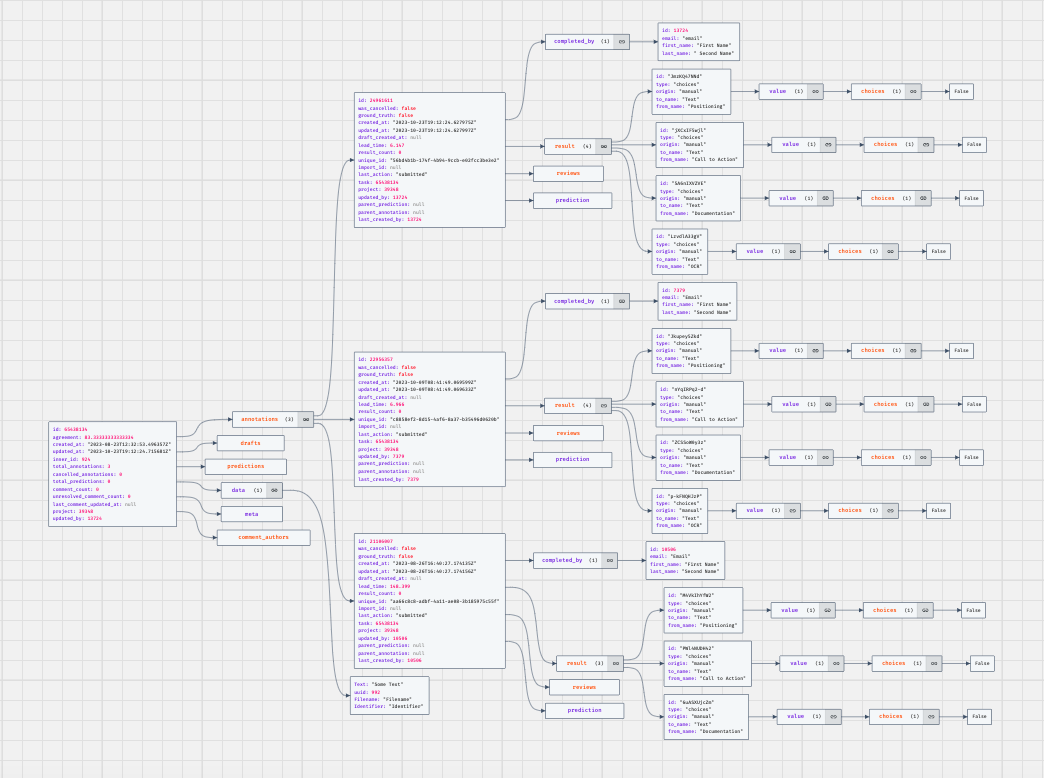
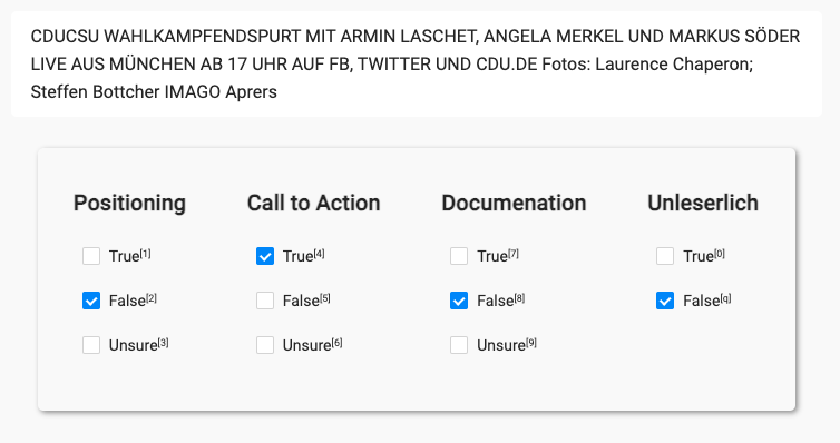
The annotations are a list of JSON objects. Each object deals with one item (e.g. one of the texts / images provided for annotation). Each object contains metadata about the annotated items, as well a list of annotation objects (in our case we expect three items).
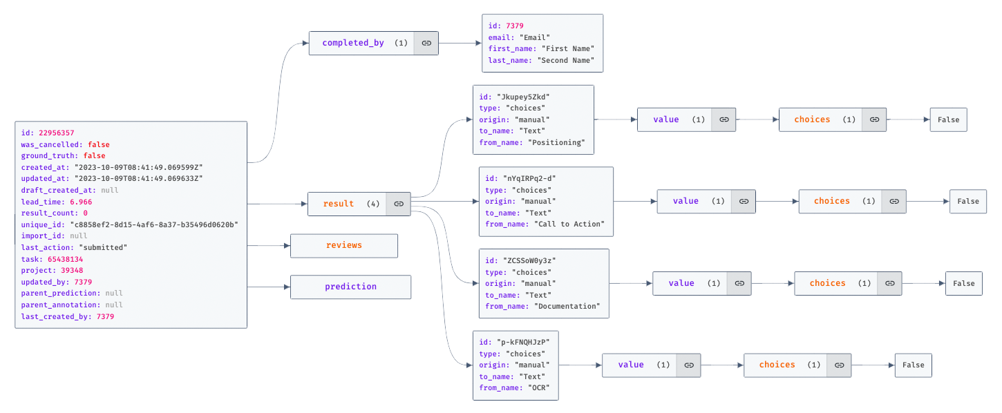
Each of these annotation objects contains one object for each coding variable, e.g. “Positioning” or “Call to Action” in our example. The actual annotation (in this case for the checkbox interface) is contained in the coding object’s child element value.choices[0].
With this structure in mind, we can start importing our annotations. The intention behind the following notebook is to work with one coding at a time. We want to create one dataframe per coding, with one row per item (=annotated text / image object), and one column per annnotator. Later on we will add another column for our computational classifications.
The Evaluation Notebook
ImportantUpdate (29. Jan. 2024)
The original notebook (below) works well with Label Studio Enterprise, where we have one annotation project handling multiple annotations per item. I created an updated second version of this notebook which handles multiple JSON files. We can use the open source version of Label Studio and create one project per annotator. Once the annotaitons were created, we export the results and use multiple JSON files in the updated notebook. Additionally, this version handles labels, annotations of bounding boxes for images.
Read the LabelStudio Annotations from file
Enter the location (e.g. on Google Drive) of your exported json file and run this cell. It loads the annotations in a long format into the variable all_annotations_df.
Warning
This version does not handle reviews!
Warning
This version has been tested with binary classifications. Other types of nominal data should work out of the box for interrater agreement, model evaluation needs some refactoring!
human_annotations_json = '/content/drive/MyDrive/2024-01-04-Text-Annotation-Sample.json' # @param {type:"string"}

import json

with open(human_annotations_json, 'r') as f:
  j = f.read()
  exported_annotations = json.loads(j)

import pandas as pd
from tqdm.notebook import tqdm

def process_result(result, coder, md):
    value_type = result.get('type', "")
    metadata = {
        **md,
        "coder": coder,
        "from_name": result.get('from_name', "")
    }
    annotations = []
    if value_type == "choices":
        choices = result['value'].get('choices', [])
        for choice in choices:
            r = {**metadata}
            r['value'] = choice
            annotations.append(r)
    elif value_type == "taxonomy":
        taxonomies = result['value'].get('taxonomy', [])
        for taxonomy in taxonomies:
            if len(taxonomy) > 1:
                taxonomy = " > ".join(taxonomy)
            elif len(taxonomy) == 1:
                taxonomy = taxonomy[0]
            r = {**metadata}
            r['value'] = taxonomy
            annotations.append(r)
    return annotations

all_annotations = []

for data in tqdm(exported_annotations):
    annotations = data.get("annotations")
    metadata = {
        **data.get("data")
    }

    for annotation in annotations:
      coder = annotation['completed_by']['id']
      results = annotation.get("result")
      if results:
        for result in results:
          all_annotations.extend(process_result(result, coder, metadata))
      else:
        print("Skipped Missing Result")


all_annotations_df = pd.DataFrame(all_annotations)
# Check the dataframe
all_annotations_df.head()| Text | uuid | Filename | Identifier | coder | from_name | value | |
|---|---|---|---|---|---|---|---|
| 0 | CDU #SOFORTPROGRAMM MITTELSTANDSPAKET WIR MACH... | 3733 | cdu/2021-09-13_15-01-28_UTC.jpg | CTxB6cMKe2U | 13724 | Positioning | True |
| 1 | CDU #SOFORTPROGRAMM MITTELSTANDSPAKET WIR MACH... | 3733 | cdu/2021-09-13_15-01-28_UTC.jpg | CTxB6cMKe2U | 13724 | Call to Action | False |
| 2 | CDU #SOFORTPROGRAMM MITTELSTANDSPAKET WIR MACH... | 3733 | cdu/2021-09-13_15-01-28_UTC.jpg | CTxB6cMKe2U | 13724 | Documentation | False |
| 3 | CDU #SOFORTPROGRAMM MITTELSTANDSPAKET WIR MACH... | 3733 | cdu/2021-09-13_15-01-28_UTC.jpg | CTxB6cMKe2U | 13724 | OCR | False |
| 4 | CDU #SOFORTPROGRAMM MITTELSTANDSPAKET WIR MACH... | 3733 | cdu/2021-09-13_15-01-28_UTC.jpg | CTxB6cMKe2U | 7379 | Positioning | True |
Contingency Table
We select one coding in this step (e.g. Positioning) and create a contingency table where each annotated item (text, image) occupies one row and each coder one column. The identifier should be set to a unique column, like uuid or Filename.
Enter the from_name for the variable you’re interested in at the moment. (Refer to your LabelStudio Interface for the right from_name).
import pandas as pd
import numpy as np

from_name = 'Positioning'
identifier = 'uuid'

filtered_df = all_annotations_df[all_annotations_df['from_name'].str.contains(from_name, case=False)]

def to_bool(val):
  if isinstance(val, bool):
    return val
  if isinstance(val, str):
    return val.lower() == "true"

  return bool(val)

values = filtered_df['value'].unique()
identifier_values = filtered_df[identifier].unique()

contingency_matrix = pd.crosstab(filtered_df[identifier], filtered_df['coder'], values=filtered_df['value'], aggfunc='first')
contingency_matrix = contingency_matrix.reindex(identifier_values)
# Let's take a look at the contigency table. We refer to each coder using a pseudonymous number.
contingency_matrix.head()| coder | 7107 | 7379 | 10506 | 13724 |
|---|---|---|---|---|
| uuid | ||||
| 3733 | NaN | True | True | True |
| 4185 | False | True | True | NaN |
| 530 | NaN | True | False | True |
| 2721 | NaN | False | False | False |
| 3384 | NaN | False | False | False |
Calculate Pairwise \(\kappa\)
Let’s calculate Cohen’s Kappa for each coder pair.
from sklearn.metrics import cohen_kappa_score

# Function to calculate Cohen's Kappa for each pair of raters
def calculate_kappa(matrix):
    raters = matrix.columns
    kappa_scores = []
    for i in range(len(raters)):
        for j in range(i+1, len(raters)):
            rater1, rater2 = raters[i], raters[j]
            # Drop NA values for the pair of raters
            pair_matrix = matrix[[rater1, rater2]].dropna()
            # Skip pairs without overlaps
            if len(pair_matrix) > 0:
              kappa = cohen_kappa_score(pair_matrix[rater1], pair_matrix[rater2])
              kappa_scores.append({
                  "Coder 1": rater1,
                  "Coder 2": rater2,
                  "Kappa": kappa,
                  "Overlap": len(pair_matrix),
                  "Coding": from_name
                  })
    return kappa_scores

kappa_scores = calculate_kappa(contingency_matrix)
kappa_scores_df = pd.DataFrame(kappa_scores)
# Let's display the pairwise Kappa agreements.
kappa_scores_df| Coder 1 | Coder 2 | Kappa | Overlap | Coding | |
|---|---|---|---|---|---|
| 0 | 7107 | 7379 | 0.469027 | 20 | Positioning |
| 1 | 7107 | 10506 | 0.782609 | 20 | Positioning |
| 2 | 7379 | 10506 | 0.669500 | 50 | Positioning |
| 3 | 7379 | 13724 | 0.888889 | 30 | Positioning |
| 4 | 10506 | 13724 | 0.714286 | 30 | Positioning |
Overall Agreement: Krippendorff’s \(\alpha\)
Next, we calculate the overall agreement using Krippendorffs Alpha. First we need to install the package.
!pip install krippendorffCollecting krippendorff
Downloading krippendorff-0.6.1-py3-none-any.whl (18 kB)
Requirement already satisfied: numpy<2.0,>=1.21 in /usr/local/lib/python3.10/dist-packages (from krippendorff) (1.23.5)
Installing collected packages: krippendorff
Successfully installed krippendorff-0.6.1import krippendorff
import pandas as pd
def convert_to_reliability_data(matrix):
transposed_matrix = matrix.T
reliability_data = []
for _, ratings in transposed_matrix.iterrows():
reliability_data.append(ratings.tolist())
return reliability_data
reliability_data = convert_to_reliability_data(contingency_matrix)
# Calculating Krippendorff's Alpha treating "Unsure" as a distinct category
alpha = krippendorff.alpha(reliability_data=reliability_data, level_of_measurement='nominal')
print("Krippendorff's Alpha:", alpha)Krippendorff's Alpha: 0.6977687626774848Majority Decision
One approach to assess the quality of machine labelled data is the comparison between machine-generated labels and human-generated labels, commonly known as “gold standard” labels. This process is called “label agreement” or “inter-rater agreement” and is widely used in various fields, including natural language processing, machine learning, and computational social science.
We are going to use create a majority_decision column using the human annotations: We have chosen an uneven number of annotators in order to find a majority for each label. First, we are going to create a contingency table (or matrix), then we can determine the majority decision.
import numpy as np
import pandas as pd

# Each row represents an item, and each column a decision from a different annotator.

# Step 1: Find the mode (most common decision) for each row
# The mode is used as it represents the majority decision.
# decisions will have the most frequent value in each row, handling ties by keeping all modes.
decisions = contingency_matrix.mode(axis=1)

# Step 2: Extract the primary mode (first column after mode operation)
# This represents the majority decision. If there's a tie, it takes the first one.
majority_decisions = decisions.iloc[:, 0]

##########
## Warning: This part needs some refactoring. Will be updated shortly.
##########
# Step 3: Count the number of non-NaN values (actual decisions) per row, excluding the first column
# Use .iloc[:, 1:] to exclude the first column
# row_non_nan_counts = contingency_matrix.iloc[:, 1:].notnull().sum(axis=1)

# Step 4: Invalidate the majority decision where the number of decisions is insufficient or even
# Majority decisions are only considered valid if there are more than 2 decisions and the number of decisions is odd.

# Define a condition for invalidating rows
# invalid_rows_condition = (row_non_nan_counts < 3) | (row_non_nan_counts % 2 == 0)


# Step 5: Append the majority decision as a new column in the contingency matrix
# This column now represents the aggregated decision from the annotators per item.
contingency_matrix['Majority Decision'] = majority_decisionscontingency_matrix.head()| coder | 7107 | 7379 | 10506 | 13724 | Majority Decision |
|---|---|---|---|---|---|
| uuid | |||||
| 3733 | NaN | True | True | True | True |
| 4185 | False | True | True | NaN | True |
| 530 | NaN | True | False | True | True |
| 2721 | NaN | False | False | False | False |
| 3384 | NaN | False | False | False | False |
Import computational annotations Reading the GPT annotations. Enter the correct file path below. coding_column needs to point to the column with you computational annotations, annotated_identifier to an id / filename that has been passed to LabelStudio project. The annotations are merged with the classifications based on annotated_identifier, in my case uuid.
annotated_file = '/content/drive/MyDrive/2024-01-04-Text-Annotation-Sample.csv'
coding_column = 'Positioning'
annotated_identifier = 'uuid'

annotated_df = pd.read_csv(annotated_file)annotated_df.head()| Unnamed: 0 | Text | Post Type | Positioning | uuid | |
|---|---|---|---|---|---|
| 0 | 54 | Gemeinsam als #eineUnion stehen wir für eine ... | Post | True | 54 |
| 1 | 200 | Wir wünschen allen Schülerinnen und Schüler... | Post | True | 200 |
| 2 | 530 | Fränkisches Essen gibt Kraft: Nach einem Mitt... | Post | False | 530 |
| 3 | 707 | Kleines Zwischenfazit zum #TvTriell. | Post | False | 707 |
| 4 | 899 | In einem paar Tagen sind Wahlen, wichtige Wahl... | Story | False | 899 |
contingency_table = pd.merge(contingency_matrix, annotated_df[['uuid', coding_column]], left_on=identifier, right_on=annotated_identifier, how='left')
contingency_table.rename(columns={coding_column: "Model"}, inplace=True)contingency_table.head()| uuid | 7107 | 7379 | 10506 | 13724 | Majority Decision | Model | |
|---|---|---|---|---|---|---|---|
| 0 | 3733 | NaN | True | True | True | True | True |
| 1 | 4185 | False | True | True | NaN | True | True |
| 2 | 530 | NaN | True | False | True | True | False |
| 3 | 2721 | NaN | False | False | False | False | False |
| 4 | 3384 | NaN | False | False | False | False | False |
Let’s suppose we’re dealing with binary data. We convert all value to binary, in order to be able to compare them correctly.
Note
The cell below needs refactoring for different type of data. In case of nominal data inside strings it might be enough to skip the cell below. A custom solution is needed for more complex use cases. Additionally, make sure to adopt the majority decision cells to any changes down here and vice versa.
# Function to convert a column to boolean if it's not already
def convert_to_bool(column):
    if contingency_table[column].dtype != 'bool':
        bool_map = {'True': True, 'False': False}
        return contingency_table[column].map(bool_map)
    return contingency_table[column]

# Convert columns to boolean if they are not already
contingency_table['Majority Decision']= convert_to_bool('Majority Decision')
contingency_table['Model'] = convert_to_bool('Model')
Let’s quickly check pairwise agreement between the Model and Majority Decision using Cohen’s Kappa:
kappa_scores = calculate_kappa(contingency_table[['Majority Decision', 'Model']])
pd.DataFrame(kappa_scores).head()| Coder 1 | Coder 2 | Kappa | Overlap | Coding | |
|---|---|---|---|---|---|
| 0 | Majority Decision | Model | 0.831461 | 50 | Positioning |
Machine Learning Metrics
Finally, let’s calculate Accuracy, Precision, and F1 Score and plot a confusion matrix.
import pandas as pd
from sklearn.metrics import accuracy_score, precision_score, recall_score, f1_score
from IPython.display import display, Markdown


# Calculating metrics
accuracy = accuracy_score(contingency_table['Majority Decision'], contingency_table['Model'])
precision = precision_score(contingency_table['Majority Decision'], contingency_table['Model'], average='binary')
recall = recall_score(contingency_table['Majority Decision'], contingency_table['Model'], average='binary')
f1 = f1_score(contingency_table['Majority Decision'], contingency_table['Model'], average='binary')

# Creating a DataFrame for the metrics
metrics_df = pd.DataFrame({
    'Metric': ['Accuracy', 'Precision', 'Recall', 'F1 Score'],
    'Value': [accuracy, precision, recall, f1]
})

# Displaying the DataFrame as a table
display(metrics_df)| Metric | Value | |
|---|---|---|
| 0 | Accuracy | 0.940000 |
| 1 | Precision | 1.000000 |
| 2 | Recall | 0.769231 |
| 3 | F1 Score | 0.869565 |
import seaborn as sns
from sklearn.metrics import confusion_matrix
import matplotlib.pyplot as plt

# Generate the confusion matrix
cm = confusion_matrix(contingency_table['Majority Decision'], contingency_table['Model'])

# Plotting the confusion matrix
plt.figure(figsize=(8, 6))
sns.heatmap(cm, annot=True, fmt='d', cmap='Blues', xticklabels=['False', 'True'], yticklabels=['False', 'True'])
plt.title('Confusion Matrix')
plt.xlabel('Predicted Label')
plt.ylabel('True Label')
plt.show()
Conclusion: Prompt Optimization
This chapter provided an overview of interrater agreement measures and machine learning model evaluation metrics. The last part of the chapter showcases the evaluation notebook, which we can use to import Label Studio annotations and calculate different types of metrics, with the ultimate goal of evaluating our model / prompt against the majority decision, our gold standard or ground truth data. The notebook can also be used throughout the prompting and classification process: Sample a smaller number of items (ca. 50-150, depending on your data) and have each member of your group annotate them. Check the interrater agreement, and in case of reasonable agreement levels use this dataset as your training dataset in an iterative process:
- Filter your dataset to only include items with training annotations.
- Run the classification for all training rows.
- Import the training annotations and training classifications in the evaluation notebook.
- Run the evaluation, check the quality, especially the confusion matrix: Can you spot any problems? Is the F1-Score reasonable?
- Optionally take a qualitative look at mislabellings. Can you spot any patterns? Take another look at prompt design ideas, e.g. use the negative examples in a conversation with ChatGPT and try to improve the prompt.
- Go back to step 2., repeat until the classification quality stagnates.
Törnberg (2024) provides further information on this process.
Warning
The term training data is possibly misleading. When training models using machine learning techinque we use sophisticated approaches to generate a training, a validation set, and a test dataset. The training dataset is used to train the model, the validation set to find the best model, and the test set to estimate the accuracy of your approach. See e.g. this medium article. Using Zero-Shot prompts for classification does not need any training data, when working with Few-Shot prompts we might consider the examples as training data as well.
Why did I chose such a misleading name? Because we need to be careful when evaluating our prompts: When optimizing the prompt following the loop above, we might possibly introduce a bias! Once the prompt has been optimized you should run a final evaluation using a larger test set to make sure that your prompt is not “overfitting”.
This chapter, in combination with the classification chapter, provides a solid foundation for computational analyses. The evaluation concept can also be applied to visual classifications: We can use Label Studio to collect the codings from our participants and evaluate them in the same fashion as shown in the evaluation notebook.
Further Reading
- Resnik and Lin (2010): Evaluation of NLP Systems, in The Handbook of Computational Linguistics and Natural Language Processing.
References
Flach, Peter. 2019. “Performance Evaluation in Machine Learning: The Good, the Bad, the Ugly, and the Way Forward.” Proceedings of the AAAI Conference on Artificial Intelligence 33 (01): 9808–14. https://doi.org/10.1609/aaai.v33i01.33019808.
Haim, Mario. 2023. Computational Communication Science: Eine Einführung. Springer Fachmedien Wiesbaden.
Klie, Jan-Christoph, Richard Eckart de Castilho, and Iryna Gurevych. 2024. “Analyzing dataset annotation quality management in the wild.” Computational Linguistics (Association for Computational Linguistics) 50 (3): 1–50. https://doi.org/10.1162/coli\_a\_00516.
Resnik, Philip, and Jimmy Lin. 2010. “Evaluation of NLP Systems.” In The Handbook of Computational Linguistics and Natural Language Processing, 271–95. Oxford, UK: Wiley-Blackwell. https://doi.org/10.1002/9781444324044.ch11.
Törnberg, Petter. 2024. “Best Practices for Text Annotation with Large Language Models.” arXiv [Cs.CL], February. http://arxiv.org/abs/2402.05129.
Reuse
Citation
BibTeX citation:
@online{achmann-denkler2024,
  author = {Achmann-Denkler, Michael},
  title = {Agreement \& {Evaluation}},
  date = {2024-12-09},
  url = {https://social-media-lab.net/evaluation/agreement.html},
  doi = {10.5281/zenodo.10039756},
  langid = {en}
}
For attribution, please cite this work as:
Achmann-Denkler, Michael. 2024. “Agreement &
Evaluation.” December 9, 2024. https://doi.org/10.5281/zenodo.10039756.