Agreement & Evaluation

Read the LabelStudio Annotations from file

Enter the location (e.g. on Google Drive) of your exported json file and run this cell. It loads the annotations in a long format into the variable all_annotations_df.

Warning

This version does not handle reviews!

Warning

This version has been tested with binary classifications. Other types of nominal data should work out of the box for interrater agreement, model evaluation needs some refactoring!

human_annotations_json = '/content/drive/MyDrive/2024-01-04-Text-Annotation-Sample.json' # @param {type:"string"}

import json

with open(human_annotations_json, 'r') as f:
  j = f.read()
  exported_annotations = json.loads(j)

import pandas as pd
from tqdm.notebook import tqdm

def process_result(result, coder, md):
    value_type = result.get('type', "")
    metadata = {
        **md,
        "coder": coder,
        "from_name": result.get('from_name', "")
    }
    annotations = []
    if value_type == "choices":
        choices = result['value'].get('choices', [])
        for choice in choices:
            r = {**metadata}
            r['value'] = choice
            annotations.append(r)
    elif value_type == "taxonomy":
        taxonomies = result['value'].get('taxonomy', [])
        for taxonomy in taxonomies:
            if len(taxonomy) > 1:
                taxonomy = " > ".join(taxonomy)
            elif len(taxonomy) == 1:
                taxonomy = taxonomy[0]
            r = {**metadata}
            r['value'] = taxonomy
            annotations.append(r)
    return annotations

all_annotations = []

for data in tqdm(exported_annotations):
    annotations = data.get("annotations")
    metadata = {
        **data.get("data")
    }

    for annotation in annotations:
      coder = annotation['completed_by']['id']
      results = annotation.get("result")
      if results:
        for result in results:
          all_annotations.extend(process_result(result, coder, metadata))
      else:
        print("Skipped Missing Result")


all_annotations_df = pd.DataFrame(all_annotations)

# Check the dataframe
all_annotations_df.head()

	Text	uuid	Filename	Identifier	coder	from_name	value
0	CDU #SOFORTPROGRAMM MITTELSTANDSPAKET WIR MACH...	3733	cdu/2021-09-13_15-01-28_UTC.jpg	CTxB6cMKe2U	13724	Positioning	True
1	CDU #SOFORTPROGRAMM MITTELSTANDSPAKET WIR MACH...	3733	cdu/2021-09-13_15-01-28_UTC.jpg	CTxB6cMKe2U	13724	Call to Action	False
2	CDU #SOFORTPROGRAMM MITTELSTANDSPAKET WIR MACH...	3733	cdu/2021-09-13_15-01-28_UTC.jpg	CTxB6cMKe2U	13724	Documentation	False
3	CDU #SOFORTPROGRAMM MITTELSTANDSPAKET WIR MACH...	3733	cdu/2021-09-13_15-01-28_UTC.jpg	CTxB6cMKe2U	13724	OCR	False
4	CDU #SOFORTPROGRAMM MITTELSTANDSPAKET WIR MACH...	3733	cdu/2021-09-13_15-01-28_UTC.jpg	CTxB6cMKe2U	7379	Positioning	True

Contingency Table

We select one coding in this step (e.g. Positioning) and create a contingency table where each annotated item (text, image) occupies one row and each coder one column. The identifier should be set to a unique column, like uuid or Filename.

Enter the from_name for the variable you’re interested in at the moment. (Refer to your LabelStudio Interface for the right from_name).

import pandas as pd
import numpy as np

from_name = 'Positioning'
identifier = 'uuid'

filtered_df = all_annotations_df[all_annotations_df['from_name'].str.contains(from_name, case=False)]

def to_bool(val):
  if isinstance(val, bool):
    return val
  if isinstance(val, str):
    return val.lower() == "true"

  return bool(val)

values = filtered_df['value'].unique()
identifier_values = filtered_df[identifier].unique()

contingency_matrix = pd.crosstab(filtered_df[identifier], filtered_df['coder'], values=filtered_df['value'], aggfunc='first')
contingency_matrix = contingency_matrix.reindex(identifier_values)

# Let's take a look at the contigency table. We refer to each coder using a pseudonymous number.
contingency_matrix.head()

coder	7107	7379	10506	13724
uuid
3733	NaN	True	True	True
4185	False	True	True	NaN
530	NaN	True	False	True
2721	NaN	False	False	False
3384	NaN	False	False	False

Calculate Pairwise \(\kappa\)

Let’s calculate Cohen’s Kappa for each coder pair.

from sklearn.metrics import cohen_kappa_score

# Function to calculate Cohen's Kappa for each pair of raters
def calculate_kappa(matrix):
    raters = matrix.columns
    kappa_scores = []
    for i in range(len(raters)):
        for j in range(i+1, len(raters)):
            rater1, rater2 = raters[i], raters[j]
            # Drop NA values for the pair of raters
            pair_matrix = matrix[[rater1, rater2]].dropna()
            # Skip pairs without overlaps
            if len(pair_matrix) > 0:
              kappa = cohen_kappa_score(pair_matrix[rater1], pair_matrix[rater2])
              kappa_scores.append({
                  "Coder 1": rater1,
                  "Coder 2": rater2,
                  "Kappa": kappa,
                  "Overlap": len(pair_matrix),
                  "Coding": from_name
                  })
    return kappa_scores

kappa_scores = calculate_kappa(contingency_matrix)
kappa_scores_df = pd.DataFrame(kappa_scores)

# Let's display the pairwise Kappa agreements.
kappa_scores_df

	Coder 1	Coder 2	Kappa	Overlap	Coding
0	7107	7379	0.469027	20	Positioning
1	7107	10506	0.782609	20	Positioning
2	7379	10506	0.669500	50	Positioning
3	7379	13724	0.888889	30	Positioning
4	10506	13724	0.714286	30	Positioning

Overall Agreement: Krippendorff’s \(\alpha\)

Next, we calculate the overall agreement using Krippendorffs Alpha. First we need to install the package.

!pip install krippendorff

Collecting krippendorff
  Downloading krippendorff-0.6.1-py3-none-any.whl (18 kB)
Requirement already satisfied: numpy<2.0,>=1.21 in /usr/local/lib/python3.10/dist-packages (from krippendorff) (1.23.5)
Installing collected packages: krippendorff
Successfully installed krippendorff-0.6.1

import krippendorff
import pandas as pd

def convert_to_reliability_data(matrix):
    transposed_matrix = matrix.T
    reliability_data = []
    for _, ratings in transposed_matrix.iterrows():
        reliability_data.append(ratings.tolist())
    return reliability_data

reliability_data = convert_to_reliability_data(contingency_matrix)

# Calculating Krippendorff's Alpha treating "Unsure" as a distinct category
alpha = krippendorff.alpha(reliability_data=reliability_data, level_of_measurement='nominal')

print("Krippendorff's Alpha:", alpha)

Krippendorff's Alpha: 0.6977687626774848

Majority Decision

One approach to assess the quality of machine labelled data is the comparison between machine-generated labels and human-generated labels, commonly known as “gold standard” labels. This process is called “label agreement” or “inter-rater agreement” and is widely used in various fields, including natural language processing, machine learning, and computational social science.

We are going to use create a majority_decision column using the human annotations: We have chosen an uneven number of annotators in order to find a majority for each label. First, we are going to create a contingency table (or matrix), then we can determine the majority decision.

import numpy as np
import pandas as pd

# Each row represents an item, and each column a decision from a different annotator.

# Step 1: Find the mode (most common decision) for each row
# The mode is used as it represents the majority decision.
# decisions will have the most frequent value in each row, handling ties by keeping all modes.
decisions = contingency_matrix.mode(axis=1)

# Step 2: Extract the primary mode (first column after mode operation)
# This represents the majority decision. If there's a tie, it takes the first one.
majority_decisions = decisions.iloc[:, 0]

##########
## Warning: This part needs some refactoring. Will be updated shortly.
##########
# Step 3: Count the number of non-NaN values (actual decisions) per row, excluding the first column
# Use .iloc[:, 1:] to exclude the first column
# row_non_nan_counts = contingency_matrix.iloc[:, 1:].notnull().sum(axis=1)

# Step 4: Invalidate the majority decision where the number of decisions is insufficient or even
# Majority decisions are only considered valid if there are more than 2 decisions and the number of decisions is odd.

# Define a condition for invalidating rows
# invalid_rows_condition = (row_non_nan_counts < 3) | (row_non_nan_counts % 2 == 0)


# Step 5: Append the majority decision as a new column in the contingency matrix
# This column now represents the aggregated decision from the annotators per item.
contingency_matrix['Majority Decision'] = majority_decisions

contingency_matrix.head()

coder	7107	7379	10506	13724	Majority Decision
uuid
3733	NaN	True	True	True	True
4185	False	True	True	NaN	True
530	NaN	True	False	True	True
2721	NaN	False	False	False	False
3384	NaN	False	False	False	False

Import computational annotations Reading the GPT annotations. Enter the correct file path below. coding_column needs to point to the column with you computational annotations, annotated_identifier to an id / filename that has been passed to LabelStudio project. The annotations are merged with the classifications based on annotated_identifier, in my case uuid.

annotated_file = '/content/drive/MyDrive/2024-01-04-Text-Annotation-Sample.csv'
coding_column = 'Positioning'
annotated_identifier = 'uuid' 

annotated_df = pd.read_csv(annotated_file)

annotated_df.head()

	Unnamed: 0	Text	Post Type	Positioning	uuid
0	54	Gemeinsam als #eineUnion stehen wir für eine ...	Post	True	54
1	200	Wir wünschen allen Schülerinnen und Schüler...	Post	True	200
2	530	Fränkisches Essen gibt Kraft: Nach einem Mitt...	Post	False	530
3	707	Kleines Zwischenfazit zum #TvTriell.	Post	False	707
4	899	In einem paar Tagen sind Wahlen, wichtige Wahl...	Story	False	899

contingency_table = pd.merge(contingency_matrix, annotated_df[['uuid', coding_column]], left_on=identifier, right_on=annotated_identifier, how='left')
contingency_table.rename(columns={coding_column: "Model"}, inplace=True)

contingency_table.head()

	uuid	7107	7379	10506	13724	Majority Decision	Model
0	3733	NaN	True	True	True	True	True
1	4185	False	True	True	NaN	True	True
2	530	NaN	True	False	True	True	False
3	2721	NaN	False	False	False	False	False
4	3384	NaN	False	False	False	False	False

Let’s suppose we’re dealing with binary data. We convert all value to binary, in order to be able to compare them correctly.

Note

The cell below needs refactoring for different type of data. In case of nominal data inside strings it might be enough to skip the cell below. A custom solution is needed for more complex use cases. Additionally, make sure to adopt the majority decision cells to any changes down here and vice versa.

# Function to convert a column to boolean if it's not already
def convert_to_bool(column):
    if contingency_table[column].dtype != 'bool':
        bool_map = {'True': True, 'False': False}
        return contingency_table[column].map(bool_map)
    return contingency_table[column]

# Convert columns to boolean if they are not already
contingency_table['Majority Decision']= convert_to_bool('Majority Decision')
contingency_table['Model'] = convert_to_bool('Model')

Let’s quickly check pairwise agreement between the Model and Majority Decision using Cohen’s Kappa:

kappa_scores = calculate_kappa(contingency_table[['Majority Decision', 'Model']])
pd.DataFrame(kappa_scores).head()

	Coder 1	Coder 2	Kappa	Overlap	Coding
0	Majority Decision	Model	0.831461	50	Positioning

Machine Learning Metrics

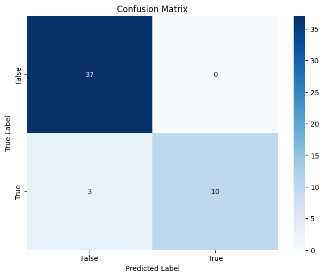
Finally, let’s calculate Accuracy, Precision, and F1 Score and plot a confusion matrix.

import pandas as pd
from sklearn.metrics import accuracy_score, precision_score, recall_score, f1_score
from IPython.display import display, Markdown


# Calculating metrics
accuracy = accuracy_score(contingency_table['Majority Decision'], contingency_table['Model'])
precision = precision_score(contingency_table['Majority Decision'], contingency_table['Model'], average='binary')
recall = recall_score(contingency_table['Majority Decision'], contingency_table['Model'], average='binary')
f1 = f1_score(contingency_table['Majority Decision'], contingency_table['Model'], average='binary')

# Creating a DataFrame for the metrics
metrics_df = pd.DataFrame({
    'Metric': ['Accuracy', 'Precision', 'Recall', 'F1 Score'],
    'Value': [accuracy, precision, recall, f1]
})

# Displaying the DataFrame as a table
display(metrics_df)

	Metric	Value
0	Accuracy	0.940000
1	Precision	1.000000
2	Recall	0.769231
3	F1 Score	0.869565

import seaborn as sns
from sklearn.metrics import confusion_matrix
import matplotlib.pyplot as plt

# Generate the confusion matrix
cm = confusion_matrix(contingency_table['Majority Decision'], contingency_table['Model'])

# Plotting the confusion matrix
plt.figure(figsize=(8, 6))
sns.heatmap(cm, annot=True, fmt='d', cmap='Blues', xticklabels=['False', 'True'], yticklabels=['False', 'True'])
plt.title('Confusion Matrix')
plt.xlabel('Predicted Label')
plt.ylabel('True Label')
plt.show()